Download
1 / 63
630 likes | 827 Vues
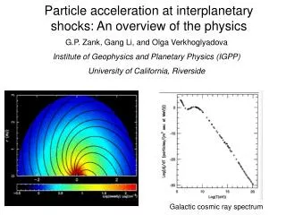
Particle acceleration at interplanetary shocks: An overview of the physics. G.P. Zank, Gang Li, and Olga Verkhoglyadova Institute of Geophysics and Planetary Physics (IGPP) University of California, Riverside. Galactic cosmic ray spectrum.

E N D
Particle acceleration at interplanetary shocks: An overview of the physics G.P. Zank, Gang Li, and Olga Verkhoglyadova Institute of Geophysics and Planetary Physics (IGPP) University of California, Riverside Galactic cosmic ray spectrum
Understanding the problem of particle acceleration at interplanetary shocks is assuming increasing importance, especially in the context of understanding the space environment. • Basic physics thought to have been established in the late 1970’s and 1980’s, but detailed interplanetary observations are not easily interpreted in terms of the simple original models of particle acceleration at shock waves. • Three fundamental aspects make the interplanetary problem more complicated than typical astrophysical problem: the time dependence of theacceleration and the solar wind background; the geometry of the shock; and the long mean free path for particle transport away from the shock. • Multiple shocks can be present simultaneously in the solar wind. • Consequently, the shock itself introduces a multiplicity of time scales, ranging from shock propagation time scales to particle acceleration time scales at parallel and perpendicular shocks, and many of these time scales feed into other time scales (such as determining maximum particle energy scalings, escape time scales, etc.).
Outline • Overview of shock acceleration at quasi-parallel shocks • Perpendicular shocks • Injection • Modeling real SEP and ESP events • Mediated shocks: some comments if time permits
Particle Acceleration – Alfven wave scattering at quasi-parallel shocks Near the shock front, Alfven waves are responsible for particle scattering. The particle distribution f, and wave energy density A are coupled together through: Bell, 1977 Gordon et al., 1999 used to evaluate wave intensity. P_max, N_inj, p_inj, s, etc. Bohm limit applied when wave energy density per log bandwidth exceeds local solar wind magnetic energy density.
The accelerated particle intensities are constant downstream of the shock and exponentially decaying upstream of the shock. • The scale length of the decay is determined by the momentum dependent diffusion coefficient (steady state solution). Diffusive shock acceleration • Trapped particles • convect • cool • diffuse. • Escaped particles • Transport to 1 AU (weak scattering).
Need to solve at the shock: Local shock accelerated distribution: Injection rate per unit areaArea of shock waveInjection momentumLocal maximum energy Spatial injection flux (particles per unit time): Young interplanetary shocks which have not yet experienced any significant deceleration inject and accelerate particles far more efficiently than do older shocks which are in a decaying phase.
a f a f z a f a f b g R t q t p max » k ¢ ¢ a f p d ln p & 2 R t u p inj 1 Timescales and particle energies • The use of the steady state solution in this time dependent model is based on the assumption that the shock wave, at a given time in the simulation, has had sufficient time to accelerate all the particles involved in the simulation. • The maximum particle energy can be determined by equating the dynamic timescale of the shock with the acceleration timescale (Drury [1983], Zank et al. 2000). 3 s = q • The acceleration time is - s 1 where giving r u = = 1 2 s r u 2 1 The maximum particle momentum obtained for a strong shock at early times can be as high as a few GeV – consistent with results obtained by Kahler [1994].
ACCELERATION TIME SCALE Particle scattering strength Hard sphere scattering: Weak scattering: Strong scattering: Acceleration time at quasi-par shock much greater than at quasi-perp shock.
Maximum particle energy at quasi-parallel shock: AgeStrengthMagnetic field heliocentric dependence
Particle acceleration at perpendicular shocks The problems: 1) High injection threshold necessary 2) No self-excited waves
TRANSVERSE COMPLEXITY Qin et al. [2002a,b] - perpendicular diffusion can occur only in the presence of a transverse complex magnetic field. Flux surfaces with high transverse complexity are characterized by the rapid separation of nearby magnetic field lines. Slab turbulence only – no development of transversely complex magnetic field. Superposition of 80% 2D and 20% slab turbulence, with the consequent development of a transversely complex magnetic field.
INTEGRAL FORM OF THE NONLINEAR GUIDING CENTER THEORY Matthaeus, Qin, Bieber, Zank [2003] derived a nonlinear theory for the perpendicular diffusion coefficient, which corresponds to a solution of the integral equation Superposition model: 2D plus slab Solve the integral equation approximately (Zank, Li, Florinski, et al, 2004): modeled according to QLT.
SHOCK U_down INTERPLANETARY MAGNETIC FIELD U_up WHAT ABOUT WAVE EXCITATION UPSTREAM? Quasi-linear theory (Lee, 1983; Gordon et al, 1999): wave excitation proportional to cos ψ i.e., at a highly perpendicular shock.
Left: Plot of the parallel (solid curve) and perpendicular mfp (dashed curve) and the particle gyroradius (dotted) as a function of energy for 100 AU (the termination shock) and 1 AU (an interplanetary shock). Right: Different format - plots of the mean free paths at 1 AU as a function of particle gyroradius and now normalized to the correlation length. The graphs are equivalent to the ratio of the diffusive acceleration time to the Bohm acceleration time, and each is normalized to gyroradius. Solid line corresponds to normalized (to the Bohm acceleration time scale) perpendicular diffusive acceleration time scale, the dashed-dotted to parallel acceleration time scale, and the dashed to Bohm acceleration time scale (obviously 1).
ANISOTROPY AND THE INJECTION THRESHOLD Diffusion tensor: Since , the anisotropy is defined by For a nearly perpendicular shock DIFFUSION APPROXIMATION VALID IF
ANISOTROPY AND THE INJECTION THRESHOLD Injection threshold as a function of angle for Anisotropy as a function of energy (r = 3) Remarks: 1)Anisotropy very sensitive to 2) Injection more efficient for quasi-parallel and strictly perpendicular shocks
PARTICLE ACCELERATION AT PERPENDICULAR SHOCKS • STEP 1: Evaluate K_perp at shock using NLGC theory instead of wave growth expression. Parallel mfp evaluated on basis of QLT (Zank et al. 1998.
PARTICLE ACCELERATION AT PERPENDICULAR SHOCKS • STEP 2: Evaluate injection momentum p_min by requiring the particle anisotropy to be small.
a f a f z a f a f b g R t q t p max » k ¢ ¢ a f p d ln p & 2 R t u p inj 1 PARTICLE ACCELERATION AT PERPENDICULAR SHOCKS • STEP 3: Determine maximum energy by equating dynamical timescale and acceleration timescale – complicated in NLGC framework. In inner heliosphere, particles resonate with inertial range (unlike outer heliosphere). Remarks: Like quasi-parallel case, p_max decreases with increasing heliocentric distance.
Remarks re maximum energies • Fundamental difference between the perpendicular and quasi-parallel expressions is that the former is derived from a quasi-linear theory based on pre-existing turbulence in the solar wind, whereas the latter results from solving the coupled wave energy and cosmic ray streaming equation explicitly, i.e., in the perpendicular case, the energy density in slab turbulence corresponds to that in the ambient solar wind whereas in the case of quasi-parallel shocks, it is determined instead by the self-consistent excitation of waves by the accelerated particles themselves. • From another perspective, unlike the quasi-parallel case, the resonance condition does not enter into the evaluation of p_max. The diffusion coefficient is fundamentally different in each case, and hence the maximum attainable energy is different for a parallel or perpendicular shock. • In the inner heliosphere where the mean magnetic field is strong, the maximum momentum decreases with increasing field strength, this reflecting the increased "tension" in the mean field.
Remarks re maximum energies – different shock configurations and ionic species Three approaches have been identified for determining p_max Zank et al 2000; Li et al 2003]. • 1. For protons accelerated at quasi-parallel shock, p_max determined purely on basis of balancing the particle acceleration time resulting from resonant scattering with the dynamical timescale of the shock. The wave/turbulence spectrum excited by the streaming energized protons extends in wave number as far as the available dynamical time allows. • 2. For heavy ions at a quasi-parallel shock, the maximum energy is also computed on the basis of a resonance condition but only up to the minimum k excited by the energetic streaming ions, which control the development of the wave spectrum. Thus, maximum energies for heavy ions are controlled by the accelerated protons and their self-excited wave spectrum. This implies a (Q/A )^2 dependence of the maximum attainable particle energy for heavy ions. • 3. For protons at a highly perpendicular shock, the maximum energy is independent of the resonance condition, depending only on the shock parameters and upstream turbulence levels. For heavy ions, this implies either a (Q/A)^{1/2} or a (Q/A)^{4/3} dependence of the maximum attainable particle energy, depending on the relationship of the maximum energy particle gyroradius compared to turbulence correlation length scale. • It may be possible to extract observational signatures related to the mass – charge ratio that distinguish particle acceleration at quasi-parallel and highly perpendicular shocks.
Maximum and injection energies Remarks: 1) Parallel shock calculation assumes wave excitation implies maximum energies comparable 3) Injection energy at Q-perp shock much higher than at Q-par therefore expect signature difference in composition
Parallel and perpendicular diffusion coefficients K_perp = black K_par = red Remarks: 1) K_par includes waves 2) The diffusion coefficients as a function of kinetic energy at various heliocentric distances. The inclusion of wave self-excitation makes K_parallel significantly smaller than K_perp at low energies, and comparable at high energies. Can utilize interplanetary shock acceleration models of Zank et al., 2000 and Li et al., 2003, 2005 for perpendicular shock acceleration to derive spectra, intensity profiles, etc.
Observations Perpendicular shock Quasi-perp shock Thanks to David Lario for particle data
CONCLUDING REMARKS FOR PERPENDICULAR SHOCKS • Developed basic theory for particle acceleration at highly perpendicular shocks based on convection of in situ solar wind turbulence into shock. • Highest injection energies needed for quasi-perp shocks and not for pure perpendicular shock. 90 degree shock singular example. • Determination of K_perp based on Nonlinear Guiding Center Theory • Maximum energies at quasi-perp shocks less than at quasi-par shocks near sun. Further from sun, reverse is true. • Injection energy threshold much higher for quasi-perp shocks than for quasi-parallel shocks and therefore can expect distinctive compositional signatures for two cases. • Observations support notion of particle acceleration at shocks in absence of stimulated wave activity.
Solar Flare vs CME-Driven Shock • The models presented here: • are one- and two-dimensional • assume acceleration takes place at the CME driven shock • are time-dependent and dynamical. • Zank et al., JGR, 105, 12,079, 2000; Li et al., JGR, 108, 1082, 2003, 2004abc; Rice et al., JGR, 108, 1369, 2003. Figures from Cliver, 2000.
Intensity profiles after Cane et al. (1988); Reames et al. (1996). Only the fastest CMEs (~1-2 %) drive shocks which make high-energy particles.
perp parallel
Particle Transport Particle transport obeys Boltzmann(Vlasov) equation: The LHS contains the material derivative and the RHS describes various “collision” processes. • Collision in this context is pitch angle scattering caused by the irregularities of IMF and in quasi-linear theory, • The result of the parallel mean free path , from a simple QLT is off by an order of magnitude from that inferred from observations, leading to a 2-D slab model. Allows a Monte-Carlo technique.
Shock speed Injection energy keV Maximum energy keV Compression ratio Particle Energies We consider three shocks: strong, intermediate, and weak.
Weak shock Strong shock Wave spectra and diffusion coefficient at shock Wave intensity Diffusion coefficient
Upstream particle spectrum(strong shock) Early time • Cumulative spectra at 1 AU for five time intervals are shown, T=1.3 days. • Spectra exhibit a power law feature. • Broken power law at later times, especially for larger mfp (λ_0 = 1.6AU). E.g., K=20 MeV for the time interval t = 4/5-1 T – particle acceleration no longer to these energies.
Intensity profiles emphasize important role of time dependent maximum energy to which protons are accelerated at a shock and the subsequent efficiency of trapping these particles in the vicinity of the shock. Compared to parallel shock case, particle intensity reaches plateau phase faster for a quasi-perpendicular shock – because K_perp at a highly perpendicular shock is larger than the stimulated K_par at a parallel shock, so particles (especially at low energies) find it easier to escape from the quasi-perpendicular shock than the parallel shock.
The time interval spectra for a perpendicular (solid line) and a parallel shock (dotted line). From left to right and top to bottom, the panels correspond to the time intervals t = (1 - {8/9})T, t = (1 - {7/9})T, … t = (1 -{1/9}) T, where T is the time taken for the shock to reach 1 AU. Note particularly the hardening of the spectrum with increasing time for the perpendicular shock example.
Event Integrated spectra Total or cumulative spectrum at 1AU, integrated over the time from shock initiation to the arrival of the shock at 1AU. Strong shock case Weak shock case Note the relatively pronounced roll-over in the cumulative strong shock spectrum and the rather flat power-law spectrum in the weak shock case.
Downstream spectra • Spectra observed at 0.8 AU at four times after the strong/inter./weak shock has passed the observer. • Note rollover at high energies (particle escape from post-shock flow) • Invariant spectra
Intensity profile (strong shock) Early time • Shock arrives 1.3 days after initiation • No K ~ 50 MeV particles at shock by 1 AU since shock weakens and unable to accelerate particles to this energy and trapped particles have now escaped. • A slowly decreasing plateau feature present –result of both pitch angle scattering and shock propagation. • Early time profile shows the brief free streaming phase.
Multiple particle crossings at 1AU Due to pitch angle scattering, particles, especially of high energies, may cross 1 AU more than once, and thus from both sides. In an average sense, a 100 MeV particle has Rc ~ 2, or on average, two crossings. Histogram shows that some particles may cross as many as 15 times. A smaller mfp leads to a larger Rc since particles with smaller mfp will experience more pitch angle scatterings.
Anisotropy at 1 AU (weak shock) • Similar to the strong shock case. • The value of asymmetry for larger λ_0 is consistently larger than that of a smaller λ_0 become fewer particles will propagate backward for a larger λ_0.
Time evolution of number density in phase space • Snap shots of the number density observed at 1 AU prior to the shock arrival at t = 1/20, 2/20, …. T, with a time interval of 1/20 T in (v_par, v_perp)-space. • Coordinates: • B field along positive Zx direction • Particle energies from innermost to outermost circle are K = 4.88, 8.12, 10.47, 15.35, 21.06, 30.75, 50.80, 100.13 MeV respectively. • The next figures exhibit the following characteristics: • At early times, more high energy particles cross 1 AU along +B direction, followed by lower energies later. • Number density of higher energy particles at later times exhibits a “reverse propagation” feature corresponding to A < 0. • The gap at Θ= 90 degree reflects that particles must have a component along B to be observed.
Phase space evolution Weak shock Strong shock
Phase space evolution – time sequence At t=0.85 T, we can see clearly that there are more backward propagating particles than forward ones between 20<K<30 MeV. At t=0.95 T, it is more pronounced for K~10 MeV.
HEAVY IONS (CNO and Fe) CNO: Q = 6, A = 14 Fe: Q = 16, A = 54 Effect of heavy ions is manifested through the resonance condition, which then determines maximum energies for different mass ions and it determines particle transport – both factors that distinguish heavy ion acceleration and transport from the proton counterpart. Shock speeds for strong and a weak shock.
Wave power and particle diffusion coefficient Strong shock example reduces to Bohm approximation. Weak shock example. The black curve is for protons, the red for CNO and the blue for Fe. The maximum energy of heavy ion shifts to lower energy end by Q/A --- a consequence of cyclotron resonance.
Deciding the maximum energy Evaluate the injection energy by assuming it is a half of the down stream thermal energy per particle. Then evaluate the maximum energy via
Maximum accelerated particle energy The maximum energy accelerated at the shock front. Particles having higher energies, which are accelerated at earlier times but previously trapped in the shock complex, will “see” a sudden change of . The maximum energy/nucleon for CNO is higher than iron since the former has a larger Q/A, thus a smaller . protons CNO Fe Bohm approximation used throughout strong shock simulation but only initially in weak shock case.