Download
1 / 80
800 likes | 1.01k Vues
PHYSTAT05 Statistical Problems in Particle Physics, Astrophysics and Cosmology Louis Lyons CDF Oxford, November 2005. History of Conferences Overview of PHYSTAT05 Specific Items Bayes and Frequentism

E N D
PHYSTAT05 Statistical Problems in Particle Physics, Astrophysics and Cosmology Louis Lyons CDF Oxford, November 2005
History of Conferences • Overview of PHYSTAT05 • Specific Items • Bayes and Frequentism • Software • Goodness of Fit • Do’s and Dont’s with Likelihoods • Systematics • Signal Significance • Where are we now ? PHYSTAT05
Issues • Bayes versus Frequentism • Limits, Significance, Future Experiments • Blind Analyses • Likelihood and Goodness of Fit • Multivariate Analysis • Unfolding • At the pit-face • Systematics and Frequentism
Talks at PHYSTAT05 7 Invited talks by Statisticians 9 Invited talks by Physicists 38 Contributed talks 8 Posters Panel Discussion 3 Conference Summaries Underlying much of the discussion: Bayes and Frequentism (Bletchley Park, Holywell Concert) 90 participants
Invited Talks by Statisticians David Cox Keynote Address: Bayesian, Frequentists & Physicists Steffen Lautitzen Goodness of Fit Jerry Friedman Machine Learning Susan Holmes Visualisation Peter Clifford Time Series Mike Titterington Deconvolution Nancy Reid Conference Summary (1/3)
Invited Talks by Physicists Bob Cousins Nuisance Parameters for Limits Kyle Cranmer LHC discovery Alex Szalay Astro + Terabytes Jean-Luc Starck Mutiscale geometry Jim Linnemann Statistical Software for Particle Physics Bob Nichol Statistical Software for Astro Stephen Johnson Historical Transits of Venus Andrew Jaffe Conference Summary (Astro) Gary Feldman Conference Summary (Particles)
Bayes versus Frequentism Old controversy Bayes 1763 Frequentism 1937 Both analyse data (x) statement about parameters ( ) e.g. Prob ( ) = 90% but very different interpretation Both use Prob (x; )
We need to make a statement about Parameters, given Data The basic difference between the two: Bayesian : Probability (parameter, given data) Anathema to a Frequentist! Frequentist : Probability (data, given parameter) (likelihood function)
PROBABILITY MATHEMATICAL Formal Based on Axioms FREQUENTIST Ratio of frequencies as n infinity Repeated “identical” trials Not applicable to single event or physical constant BAYESIANDegree of belief Can be applied to single event or physical constant (even though these have unique truth) Varies from person to person Quantified by “fair bet”
Bayesian Bayes’ Theorem posterior likelihood prior Problems: P(param) True or False “Degree of belief” Prior What functional form? Flat? Which variable? Unimportant when “data overshadows prior” Important for limits
Data overshadows Prior Prior L MZ = 91188 ± 2 MeV
Data upper limit on signal s Choice of prior affects limit prior~1/s LpriorL s s
Mass squared of νe “L” M2 Prior N.B. Posterior
P (Data;Theory) P (Theory;Data) HIGGS SEARCH at CERN Is data consistent with Standard Model? or with Standard Model + Higgs? End of Sept 2000: Data not very consistent with S.M. Prob (Data ; S.M.) < 1% valid frequentist statement Turned by the press into: Prob (S.M. ; Data) < 1% and therefore Prob (Higgs ; Data) > 99% i.e. “It is almost certain that the Higgs has been seen”
P (Data;Theory) P (Theory;Data) Theory = male or female Data = pregnant or not pregnant P (pregnant ; female) ~ 3% but P (female ; pregnant) >>>3%
Frequentist: Neyman Construction µ x x0 µ = Theoretical parameter x = ObservationNO PRIOR INVOLVED
at 90% confidence Frequentist Bayesian
Bayes versus Frequentism BayesianFrequentist
Bayes versus Frequentism Bayesian Frequentist
Bayesianism versus Frequentism “Bayesians address the question everyone is interested in, by using assumptions no-one believes” “Frequentists use impeccable logic to deal with an issue of no interest to anyone”
Statistical Software Linnemann Software for Particles Nichol Software for Astro Le Diberder sPlot Paterno R Kreschuk ROOT Verkerke RooFit Pia Goodness of Fit Buckley CEDAR Narsky StatPatternRecognition Recommendation of Statistical Software Repository at FNAL
Goodness of Fit • Basic problem: • Very general applicability, but • Requires binning, with > 5…..20 events per bin. Prohibitive with sparse data in several dimensions. • Not sensitive to signs of deviations X K-S and related tests overcome these, but work in 1-D So, need something else.
Goodness of Fit Talks Lauritzen Invited talk Yabsley GOF and sparse multi-D data Ianni GOF and sparse multi-D data Raja GOF and L Gagunashili and weighting Pia Software Toolkit for Data Analysis Block Rejecting outliers Bruckman Alignment Blobel Tracking
Goodness of Fit Gunter Zech “Multivariate 2-sample test based on logarithmic distance function” See also: Aslan & Zech, Durham Conf., “Comparison of different goodness of fit tests” R.B. D’Agostino & M.A. Stephens, “Goodness of fit techniques”, Dekker (1986)
DO’S AND DONT’S WITH L • NORMALISATION OF L • JUST QUOTE UPPER LIMIT • (ln L) = 0.5 RULE • Lmax AND GOODNESS OF FIT • BAYESIAN SMEARING OF L • USE CORRECT L (PUNZI EFFECT)
NORMALISATION OFL - t t / t = P ( t | ) e t Missing 1 / MUST be independent of m data param e.g. Lifetime fit to t1, t2,………..tn INCORRECT t
2) QUOTING UPPER LIMIT “We observed no significant signal, and our 90% conf upper limit is …..” Need to specify method e.g. L Chi-squared (data or theory error) Frequentist (Central or upper limit) Feldman-Cousins Bayes with prior = const, “Show your L” 1) Not always practical 2) Not sufficient for frequentist methods
90% C.L. Upper Limits m x x0
ΔlnL = -1/2 rule If L(μ) is Gaussian, following definitions of σ are equivalent: 1) RMS of L(µ) 2) √(-d2L/dµ2) 3) ln(L(μ±σ) = ln(L(μ0)) -1/2 If L(μ) is non-Gaussian, these are no longer the same “Procedure 3) above still gives interval that contains the true value of parameter μ with 68% probability” Heinrich: CDF note 6438 (see CDF Statistics Committee Web-page) Barlow: Phystat05
COVERAGE How often does quoted range for parameter include param’s true value? N.B. Coverage is a property of METHOD, not of a particular exptl result Coverage can vary with Study coverage of different methods of Poisson parameter , from observation of number of events n Hope for: 100% Nominalvalue
COVERAGE If true for all : “correct coverage” P< for some “undercoverage” (this is serious !) P> for some “overcoverage” Conservative Loss of rejection power
Coverage : L approach (Not frequentist) P(n,μ) = e-μμn/n! (Joel Heinrich CDF note 6438) -2 lnλ< 1 λ = P(n,μ)/P(n,μbest) UNDERCOVERS
Frequentist central intervals, NEVER undercovers(Conservative at both ends)
Feldman-Cousins Unified intervalsFrequentist, so NEVER undercovers
= (n-µ)2/µ Δ = 0.1 24.8% coverage? • NOT frequentist : Coverage = 0% 100%
Lmax and Goodness of Fit? Find params by maximising L So larger L better than smaller L So Lmax gives Goodness of Fit?? Bad Good? Great? Monte Carlo distribution of unbinned Lmax Frequency Lmax
Not necessarily: pdf L(data,params) fixed vary L Contrast pdf(data,params) param vary fixed data e.g. Max at t = 0 Max at pL tλ
Example 1 Fit exponential to times t1, t2 ,t3 ……. [Joel Heinrich, CDF 5639] L = lnLmax = -N(1 + ln tav) i.e. Depends only on AVERAGE t, but is INDEPENDENT OF DISTRIBUTION OF t (except for……..) (Average t is a sufficient statistic) Variation of Lmax in Monte Carlo is due to variations in samples’ average t , but NOT TO BETTER OR WORSE FIT pdf Same average t same Lmax t
Example 2 L = cos θ pdf (and likelihood) depends only on cos2θi Insensitive to sign of cosθi So data can be in very bad agreement with expected distribution e.g. all data with cosθ< 0 and Lmax does not know about it. Example of general principle
Example 3 Fit to Gaussian with variable μ, fixed σ lnLmax = N(-0.5 ln2π – lnσ) – 0.5 Σ(xi – xav)2 /σ2 constant ~variance(x) i.e. Lmax depends only on variance(x), which is not relevant for fitting μ (μest = xav) Smaller than expected variance(x) results in larger Lmax x x Worse fit, larger Lmax Better fit, lower Lmax
Lmax and Goodness of Fit? Conclusion: L has sensible properties with respect to parameters NOT with respect to data Lmax within Monte Carlo peak is NECESSARY not SUFFICIENT (‘Necessary’ doesn’t mean that you have to do it!)
Binned data and Goodness of Fit using L-ratio niL = μi Lbest x ln[L-ratio] = ln[L/Lbest] large μi -0.5c2 i.e. Goodness of Fit μbest is independent of parameters of fit, and so same parameter values from L or L-ratio Baker and Cousins, NIM A221 (1984) 437
L and pdf Example 1: Poisson pdf = Probability density function for observing n, given μ P(n;μ) = e -μμn/n! From this, construct L as L(μ;n) = e -μμn/n! i.e. use same function of μ and n, but . . . . . . . . . . pdf for pdf, μ is fixed, but for L, n is fixed μL n N.B. P(n;μ) exists only at integer non-negative n L(μ;n) exists only as continuous fn of non-negative μ
Example 2 Lifetime distribution pdf p(t;λ) = λ e -λt So L(λ;t) = λ e –λt(single observed t) Here both t and λ are continuous pdf maximises at t = 0 L maximises at λ = t N.B. Functionalform of P(t) and L(λ) are different Fixed λ Fixed t p L t λ
Example 3: Gaussian N.B. In this case, same functional form for pdf and L So if you consider just Gaussians, can be confused between pdf and L So examples 1 and 2 are useful
Transformation properties of pdf and L Lifetime example: dn/dt = λ e –λt Change observable from t to y = √t So (a) pdf changes, BUT (b) i.e. corresponding integrals of pdf are INVARIANT