Download
1 / 73
740 likes | 919 Vues
Serial protocols. RS-232 (IEEE standard) serial protocol for point-to-point, low-cost, low-speed applications for PCs I2C (Philips) TWI (Atmel) up to 400Kbits/sec, serial bus for connecting multiple components Ethernet (popularized by Xerox)

E N D
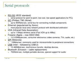
Serial protocols • RS-232 (IEEE standard) • serial protocol for point-to-point, low-cost, low-speed applications for PCs • I2C (Philips) TWI (Atmel) • up to 400Kbits/sec, serial bus for connecting multiple components • Ethernet (popularized by Xerox) • most popular local area network protocol with distributed arbitration • IrDA (Infrared Data Association) • up to 115kbps wireless serial (Fast IrDA up to 4Mbs) • Firewire (Apple – now IEEE1394) • 12.5-50Mbytes/sec, consumer electronics (video cameras, TVs, audio, etc.) • SPI (Motorola) • 10Mbits/sec, commonly used for microcontroller to peripheral connections • USB (Intel – followed by USB-2) • 12-480Mbits/sec, isochronous transfer, desktop devices • Bluetooth (Ericsson – cable replacement) • 700Kbits/sec, multiple portable devices, special support for audio Communication
RS-232 (standard serial line) • Point-to-point, full-duplex • Synchronous or asynchronous • Flow control • Variable baud (bit) rates • Cheap connections (low-quality and few wires) • Variations: parity bit; 1.5 or 2 stop bits (not common) At 9600 baud, each bit (start, data, stop) lasts 1/9600s 8 databits start bit(always low) stop bit(always high) paritybit Communication
RS-232 HW all wires active lowSpec: "0" = -3v to -15v "1" = +3v to +15vReality: even more variability PC serial port: +5 and –9 special driver chips (eg Max 232)generate high /-vevoltages from 5v or 3v Often you see “TTL level serial,” between chips or boards, +5v and 0v or +3.3v and 0v Often implemented as “virtual COMM” port over USB, e.g. FTDI chip Connector: DB-9 (old school) Wires (Spec): • TxD– transmit data • TxC – transmit clock • RTS – request to send • CTS – clear to send • RxD – receive data • RxC – receive clock • DSR – data set ready • DTR – data terminal ready • Ground Wires (Typical) • TxD, RxD, GND Communication
Transfer modes • Synchronous • clock signal wire is used by both receiver and sender to sample data • Asynchronous • no clock signal in common • data must be oversampled (16x is typical) to find bit boundaries • Flow control • handshaking signals to control rate of transfer Communication
Electric Field Sensing • Use software to make sensitive measurements • Case study: electric field sensing • You will build an electric field sensor in lab • Non-contact hand measurement (like magic!) • Software (de)-modulation for very sensitive measurements • Same basic measurement technique used in accelerometers, etc • Good intro to principles of radio • We will get signal-to-noise gain by software operations • We will need • some basic electronics • some math facts • some signal processing Interfacing
Electrosensory Fish • Weakly electric fish generate and sense electric fields • Measure conductivity “images” • Frequency range .1Hz – 10KHz Tail curling for active scan Black ghost knife fish(Apteronotus albifrons) Continuous wave, 1KHz W. Heiligenberg. Studies of Brain Function, Vol. 1: Principles of Electrolocation and Jamming Avoidance Springer-Verlag, New York, 1977. Interfacing
Electric Field Sensing for input devices Interfacing
Cool stuff you can do with E-Field sensing Interfacing
Basic electronics • Voltage sources, current sources, and Ohm’s law • AC signals • Resistance, capacitance, inductance, impedance • Op amps • Comparator • Current (“transimpedance”) amplifier • Inverting amplifier • Differentiator • Integrator • Follower Interfacing
Voltage & Current sources • “Voltage source” • Example: microcontroller output pin • Provides defined voltage (e.g. 5V) • Provides current too, but current depends on load (resistance) • Imagine a control system that adjusts current to keep voltage fixed • “Current source” • Example: some transducers • Provides defined current • Voltage depends on load • Ohm’s law (V=IR) relates voltage, current, and load (resistance) Interfacing
Ohm’s law and voltage divider Need 3 physics facts: • 1. Ohm’s law: V=IR (I=V/R) • Microcontroller output pin at 5V, 100K load I=5V/100K = 50mA • Microcontroller output pin at 5V, 200K load I=5V/200K = 25mA • Microcontroller output pin at 5V, 1K load I=5V/1K = 5mA • 2. Resistors in series add • 3. Current is conserved (“Kirchoff’s current law”) Voltage divider • Lump 2 series resistors together (200K) • Find current through both: I=5V/200K=25mA • Now plug this I into Vd=IR for 2nd resistor • Vd=25mA * 100K = 25*10-6 * 105 = 2.5V • General voltage divider formula: Vd=VR2/(R1+R2) Vd=? Interfacing
Capacitor • Apply a voltage • Creates difference in charge between two plates • Q = CV • If you change the voltage, the charge on the plates changes…apply an AC (continuously changing) voltage, get continuously changing charge == AC current
Time domain capacitor behavior “5RC rule”: a cap charges/ decays to within 1% of its final value within 5 RC time constants
e-cap.html Capacitor charge/discharge
Applications of capacitors • Energy • Supercaps ~1F • electrolytics (polarized [+-] leads! don’t hook them up backward or the smoke will escape!) ~10uF-100uF • Power supply filtering • 10uF-100uF electrolytic • “AC coupling” between amp stages • “Bypass” • 0.1uF ceramic or polyester, one per chip, shunts noise to ground • Timing and waveform generation [“delay circuits”] • Hi/low pass filtering • Differentiation (AoE1.14) / integration (AoE 1.15)
Operational amplifiers • Amplify voltages (increase voltage) • Turn weak (“high impedance”) signal into robust (“low impedance”) signal by adding current (and thus power) • Perform mathematical operations on signals (in analog) • E.g. sum, difference, differentiation, integration, etc • Originally analog computing building blocks!
Operational amplifier (as comparator) e-opamp.html
Op Amp Behavior • Op amp has two inputs, +ve & -ve. • Rule 1: Inputs are “sense only”…no current goes into the inputs • It amplifies the difference between these inputs • With a feedback network in place, it tries to ensure: • Rule 2: Voltage on inputs is equal • ensuring this is what the op-amp does! • as if inputs are shorted together…“virtual short” • more common term is “virtual ground,” but this is less accurate • Using rules 1 and 2 we can understand what op amps do
Vout +15V V- V+ -15V Comparator • Used in earlier ADC examples • No feedback (so Rule 2 won’t apply) • Vout = T{g*(V+ - V-)} [g big, say 106] • T{ } means threshold s.t. Vout doesn’t exceed rails • In practice • V+ > V- Vout = +15 • V+ < V- Vout = -15
Op amp with feedback e-opampfeedback.html
Follower • Because of direct connection, V- = Vout • Rule 2V- = V+, so • Vout = Vin Vout Vin • No current into inputs • V- = V+
Follower e-amp-follower-outputimped.html
End of lecture Interfacing
Op Amp Behavior • Op amp has two inputs, +ve & -ve. • Rule 1: Inputs are “sense only”…no current goes into the inputs • It amplifies the difference between these inputs • With a feedback network in place, it tries to ensure: • Rule 2: Voltage on inputs is equal • ensuring this is what the op-amp does! • as if inputs are shorted together…“virtual short” • more common term is “virtual ground,” but this is less accurate • Using rules 1 and 2 we can understand what op amps do
Transimpedance amp V- • Produces output voltage proportional to input current • AGND = V+ = 0V • By 2, V- = V+, so V- = 0V • Suppose Iin = 1mA • By 1, no current enters inverting input • All current must go through R1 • Vout-V- = -1mA * 106 W • Vout = -1V • Generally, Vout = - Iin * R1 Iin Vout V+ • No current into inputs • V- = V+
e-itov.html Transimpedance amp (current to voltage)
Inverting op amp e-amp-invert.html
Op Amp power supply • Dual rail: 2 pwr supplies, +ve & -ve • Can handle negative voltages • “old school” • Single supply op amps • Signal must stay positive • Use Vcc/2 as “analog ground” • Becoming more common now, esp in battery powered devices • Sometimes good idea to buffer output of voltage divider with a follower Ground 0V Dual rail op-amp 2.5V “analog ground” Single supply op-amp
End of basic electronics Interfacing
+1 -1 Electric Field Sensing circuit • For nsamps desired integration • Assume square wave TX (+1, -1) • After signal conditioning, signal goes direct to ADC • Acc = sum_i T_i * R_i • When TX high, acc = acc + sample • When TX low, acc = acc - sample ADC IN Square wave out Microcontroller Interfacing
E-Field lab pseudo-code // Set P1.0 as output// Set ADC0 as input; configure ADCNSAMPS = 200; // Try different values of NSAMPS //Look at SNR/update rate tradeoffacc = 0; // acc should be a 16 bit variableFor (i=0; i<NSAMPS; i++) { SET P1.0 HIGHacc = acc + ADCVALUE SET P1.0 LOWacc = acc - ADCVALUE}Return acc Why is this implementing inner product correlation? Imagine unrolling the loop. We’ll write ADC1, ADC2, ADC3, … for the 1st, 2nd, 3rd, … ADCVALUE acc = ADC1 – ADC2 + ADC3 – ADC4 + ADC5 – ADC6 +… acc = +1*ADC1 + -1*ADC2 + +1*ADC3 + -1*ADC4 +… acc = C1*ADC1 + C2*ADC2 + C3*ADC3 + C4*ADC4 + … where Ci is the ith sample of the carrier acc = <C,ADC> Inner product of the carrier vector with the ADC sample vector Interfacing Vectors bold, blue
Vectors! • Think of a signal as a vector of samples • Vector lives in a vector space, defined by bases • Same vector can be represented in different bases • A vector v can be projected onto various basis vectors to find out “how much” of each basis vector is in v <1,2> <2.236,0> v v Vector vin some basis Vector vin another basis Length: Sqrt(12+22)=2.236 Length: Sqrt(2.2362)=2.236 Interfacing
Vectors and modulation S’pose m and n are orthogonal unit vectors. Then inner products (dot products) are <m,m>=1 <n,n>=1 <m,n>=<n,m>=0 Can interpret inner product as projection of vector 1 (“v1”) onto vector 2 (“v2”)…in other words, inner product of v1and v2tells us “how much of vector 1 is there in the direction of vector 2.” Vectors: bold blue Scalars: not If a channel lets me send 2 orthogonal vectors through it, then I can send two independent messages. Say I need to send two numbers, a and b…I can send am+bn through the channel. At the receive side I get am+bn Now I project onto m and onto n to get back the numbers: <am+bn, m>=<am,m> + <bn, m>=a+0=a <am+bn, n>=<am,n> + <bn, n>=0+b=b The initial multiplication is modulation; the projection to separate the signals is demodulation. Each channel sharing schemea set of basis vectors. Interfacing
Physical set up for multiplexed sensing TX Electrode TX Electrode RCV Electrode Amp Micro • We can measure multiple sense channels simultaneously, sharing 1 • RCV electrode, amp, and ADC! • Choice of TX wave forms determines multiplexing method: • TDMA --- Time division: TXs take turns • FDMA --- Frequency division: TXs use different frequencies • CDMA ---- Code division: TXs use different coded waveforms • In all cases, what makes it work is ~orthogonality of the TX waveforms! Interfacing
h A D C C C A D C < > a c c = = ; ( ) h h h d d l d h l h C C i t £ a w c c e r e a n s s e n s e v a u e a n m e a n s s c a a r v e c o r h C C < > = ; h C C < > = ; h = f C C i 1 < > = ; Review Where C is the carrier vector and ADC is the vector of samples. Let’s write out ADC: Interfacing
1 1 2 2 h h A D C C C + = a c c 1 C A D C < > = ; 1 1 1 2 2 h h C C C + < > = ; 1 1 1 1 2 2 h h C C C C + < > < > = ; ; 1 1 1 2 1 2 h h C C C C + < > < > = ; ; 1 h = 1 1 1 2 f d C C C C i 1 0 < > < > a n = = ; ; Multi-access communication / sensingAbstract view Suppose we have two carriers, C1 and C2 And suppose they are orthogonal, so that < C1, C2 >=0 The received signal is Let’s demodulate with C1: Interfacing
TDMAAbstract view Verify that <C1,C2>=0 Modulated carriers Sum of modulated carriers <C1, .2C1 +.7C2>= <C1, .2C1> +<C1,.7C2>= .2 <C1, C1> + 0 Horizontal axis: time Vertical axis: amplitude (arbitrary units) Interfacing
FDMAAbstract view >> n1=sum(c1 .* c1) n1 = 2.5000e+003 >> n2=sum(c2 .* c2) n2 = 2.5000e+003 >> n12=sum(c1 .* c2) n12 = -8.3900e-013 >> rcv = .2*c1 + .7*c2; >> sum(c1/n1 .* rcv) ans = 0.2000 >> sum(c2/n2 .* rcv) ans = 0.7000 Horizontal axis: time Vertical axis: amplitude (arbitrary units) Interfacing
CDMA S’pose we pick random carriers: c1 = 2*(rand(1,500)>0.5)-1; >> n1=sum(c1 .* c1) n1 = 5000 >> n2=sum(c2 .* c2) n2 = 5000 >> n12=sum(c1 .* c2) n12 = -360 >> rcv = .2*c1 + .7*c2; >> sum(c1/n1 .* rcv) ans = 0.1496 >> sum(c2/n2 .* rcv) ans = 0.6856 Horizontal axis: time Vertical axis: amplitude (arbitrary units) Note: Random carriers here consist of 500 rand values repeated 10 times each for better display Interfacing
LFSRs (Linear Feedback Shift Registers)The right way to generate pseudo-random carriers for CDMA • A simple pseudo-random number generator • Pick a start state, iterate • Maximum Length LFSR visits all states before repeating • Based on primitive polynomial…iterating LFSR equivalent to multiplying by generator for group • Can analytically compute auto-correlation • This form of LFSR is easy to compute in HW (but not as nice in SW) • Extra credit: there is another form that is more efficient in SW • Totally uniform auto-correlation Image source: wikipedia Image source: wikipedia Interfacing
LFSR TX 8 bit LFSR with taps at 3,4,5,7 (counting from 0). Known to be maximal. for (k=0;k<3;k++) { // k indexes the 4 LFSRs low=0; if(lfsr[k]&8) // tap at bit 3 low++; // each addition performs XOR on low bit of low if(lfsr[k]&16) // tap at bit 4 low++; if(lfsr[k]&32) // tap at bit 5 low++; if(lfsr[k]&128) // tap at bit 7 low++; low&=1; // keep only the low bit lfsr[k]<<=1; // shift register up to make room for new bit lfsr[k]&=255; // only want to use 8 bits (or make sure lfsr is 8 bit var) lfsr[k]|=low; // OR new bit in } OUTPUT_BIT(TX0,lfsr[0]&1); // Transmit according to LFSR states OUTPUT_BIT(TX1,lfsr[1]&1); OUTPUT_BIT(TX2,lfsr[2]&1); OUTPUT_BIT(TX3,lfsr[3]&1); Interfacing
LFSR demodulation meas=READ_ADC(); // get sample…same sample will be processed in different ways for(k=0;k<3;k++) { if(lfsr[k]&1) // check LFSR state accum[k]+=meas; // make sure accum is a 16 bit variable! else accum[k]-=meas; } Interfacing
LFSR state sequence >> lfsr1(1:255) ans = 2 4 8 17 35 71 142 28 56 113 226 196 137 18 37 75 151 46 92 184 112 224 192 129 3 6 12 25 50 100 201 146 36 73 147 38 77 155 55 110 220 185 114 228 200 144 32 65 130 5 10 21 43 86 173 91 182 109 218 181 107 214 172 89 178 101 203 150 44 88 176 97 195 135 15 31 62 125 251 246 237 219 183 111 222 189 122 245 235 215 174 93 186 116 232 209 162 68 136 16 33 67 134 13 27 54 108 216 177 99 199 143 30 60 121 243 231 206 156 57 115 230 204 152 49 98 197 139 22 45 90 180 105 210 164 72 145 34 69 138 20 41 82 165 74 149 42 84 169 83 167 78 157 59 119 238 221 187 118 236 217 179 103 207 158 61 123 247 239 223 191 126 253 250 244 233 211 166 76 153 51 102 205 154 53 106 212 168 81 163 70 140 24 48 96 193 131 7 14 29 58 117 234 213 170 85 171 87 175 95 190 124 249 242 229 202 148 40 80 161 66 132 9 19 39 79 159 63 127 255 254 252 248 240 225 194 133 11 23 47 94 188 120 241 227 198 141 26 52 104 208 160 64 128 1 Interfacing
LFSR output >> c1(1:255) (EVEN LFSR STATE -1, ODD LFSR STATE +1) ans = -1 -1 -1 1 1 1 -1 -1 -1 1 -1 -1 1 -1 1 1 1 -1 -1 -1 -1 -1 -1 1 1 -1 -1 1 -1 -1 1 -1 -1 1 1 -1 1 1 1 -1 -1 1 -1 -1 -1 -1 -1 1 -1 1 -1 1 1 -1 1 1 -1 1 -1 1 1 -1 -1 1 -1 1 1 -1 -1 -1 -1 1 1 1 1 1 -1 1 1 -1 1 1 1 1 -1 1 -1 1 1 1 -1 1 -1 -1 -1 1 -1 -1 -1 -1 1 1 -1 1 1 -1 -1 -1 1 1 1 1 -1 -1 1 1 1 -1 -1 1 1 -1 -1 -1 1 -1 1 1 -1 1 -1 -1 1 -1 -1 -1 1 -1 1 -1 -1 1 -1 1 -1 1 -1 -1 1 1 1 -1 1 1 1 -1 1 1 -1 -1 1 1 1 1 -1 1 1 1 1 1 1 -1 1 -1 -1 1 1 -1 -1 1 1 -1 1 -1 1 -1 -1 -1 1 1 -1 -1 -1 -1 -1 1 1 1 -1 1 -1 1 -1 1 -1 1 1 1 1 1 -1 -1 1 -1 1 -1 -1 -1 -1 1 -1 -1 1 1 1 1 1 1 1 1 -1 -1 -1 -1 1 -1 1 1 1 1 -1 -1 -1 1 1 -1 1 -1 -1 -1 -1 -1 -1 -1 1 Interfacing
CDMA by LFSR >> n1 = sum(c1.*c1) n1 = 5000 >> n2 = sum(c2.*c2) n2 = 5000 >> n12 = sum(c1.*c2) n12 = -60 >> rcv = .2 *c1 + .7*c2; >> sum(c1/n1 .* rcv) ans = 0.1916 >> sum(c2/n2 .* rcv) ans = 0.6976 Note: CDMA carriers here consist of 500 pseudorandom values repeated 10 times each for better display Interfacing
Autocorrelation of pseudo-random (non-LFSR) sequence of length 255 PR seq Generated w/ Matlab rand cmd Interfacing
-1 Autocorrelation (full length 255 seq) Interfacing