
Chapter 3 Brute Force
E N D
Presentation Transcript
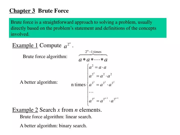
Example 1 Compute . Brute force algorithm: A better algorithm: Chapter 3 Brute Force Brute force is a straightforward approach to solving a problem, usually directly based on the problem’s statement and definitions of the concepts involved. Example 2 Search x from n elements. Brute force algorithm: linear search. A better algorithm: binary search.
Example 3 Sort n elements. (1) Selection Sort Find the smallest element and exchange it with the element in the first position, find the second smallest element and exchange it with the one in the second position, continue in this way until the entire array is sorted. Program 1 Selection sort (sort array a[1..n]) Procedure seletion(a[1..n]) { for (i=1; i < n; i++) { min = i; for ( j=i+1; j <=n; j++) if (a[j] < a[min]) min = j; exch(a[i], a[min]); } } Selection sort: l x e a m e p a x e l m e p a e x l m e p a e e l m x p a e e l m x p a e e l m x p a e e l m p x Section sort is a stable sort
Running Time of Section Sort • case • case (n-1) comparisons (n-1) comparisons (n-2) comparisons (n-2) comparisons (n-3) comparisons (n-3) comparisons Running time does not depend on the state of the input.
(2) Insertion Sort Consider the elements one at a time, inserting each into its proper place among these already considered (keeping them sorted). Sort Program 2 Insertion sort (sort array a[1..n]) Procedure insertion(a[1..n]) { for (i = 2; i<=n; i++) { j = i; v = a[i]; while (v < a[j-1]) { a[j] = a[j-1]; j--; } a[j] = v; } } m a x e l e p a m x e l e p a m x e l e p a e m x l e p a e m l x e p a e e l m x p a e e l m p x Insertion Sort is a stable sort.
Running Time of Insertion Sort • case • case 1 comparison 1 comparisons 1 comparison 2 comparisons 1 comparison 3comparisons 1 comparison (n-1) comparisons Running time depends on the state of the input. In the worst case, the running time is Better Algorithms can solve sorting problem in O(nlogn) time.
2 a b 3 8 7 5 c d 1 Example 4 Problems using exhaustive search (1) Traveling sales man problem Given a graph G, find the shortest simple circuit (Hamiltonian circuit) in G which passes through all the vertices. Tour length abcda 18 abdca 11 … Totally there are P(4,4)=4! tours. Generally, there may have n! tours in a graph of n vertices and if we check all the tours the computing time is O(n!). People couldn’t find a good algorithm (using polynomial time) to solve it!
(2) Knapsack problem knapsack: W=10 item 1: w=7, v=$42 item 2: w=3, v=$12, item 3: w=4, v= $40, item 4: w=5, v=$25 People couldn’t find a good algorithm (using polynomial time) to solve it ! The problems which people could not find polynomial algorithms for are called as NP-hard problems.
Chapter 4 Divide-and-Conquer • Divide-and-conquer: one of the most important technique used for designing algorithms • Divide a large problem into subproblems of about the same size • Solve each of subproblems • Merge the solutions of the subproblems to that of original one. Example 1 Quick sort • Quick sort n elements in array a[1..n] • Partition array a[1..n] to two parts: one whose elements is smaller than a[n] and one whose elements are larger than a[n]. • Quick sort the first part and then quick sort the second part. • Output the first part, a[n], then outputthe second part.
Program 2 Partitioning Function partition(a,l,r) return a value i such that after partitioning a[i]=v, the elements a[l..i-1] are smaller than v, and the elements a[i+1..r] are larger than v. void partition(int a[], int l, int r) { int i = l-1, j = r; Item v = a[r]; for (; ;) { while (a[++i] < v); while (v < a[--j]) if (j == 1) break; if (i >= j) break; exch(a[i],a[j]); } exch(a[i],a[r]); return i; } Program 1 Quicksort Sort a[l..r], where v=a[r]. Function partition(a,l,r) return a value i such that after partitioning a[i]=v, the elements a[l..i-1] are smaller than v, and the elements a[i+1..r] are larger than v. void quicksort(int a[], int l, int r) { if (r <= l) return; int i = partition(a, l, r); quicksort(a,l,i-1); quicksort(a,i+1,r); } the number for comparisons is n when partition a[1..n]
Less than or equal to v Greater than or equal to v r l i j 11, 6, 15, 7, 9, 18, 9, 5 , 17, 14 11, 6, 15, 7, 9, 18, 9, 5, 17, 14 v 11, 6, 15, 7, 9, 18, 9, 5, 17, 14 i i i i j i i i j j j j j j j i 11, 6, 5, 7, 9, 18, 9, 15, 17, 14 11, 6, 5, 7, 9, 18, 9, 15, 17, 14 11, 6, 5, 7, 9, 18, 9, 15, 17, 14 11, 6, 5, 7, 9, 9, 18, 15, 17, 14 11, 6, 5, 7, 9, 9, 18, 15, 17, 14 Program 2 Partitioning Function partition(a,l,r) return a value i such that after partitioning a[i]=v, the elements a[l..i-1] are smaller than v, and the elements a[i+1..r] are larger than v. void partition(int a[], int l, int r) { int i = l-1, j = r; Item v = a[r]; for (; ;) { while (a[++i] < v); while (v < a[--j])if (j == l) break; if (i >= j) break; exch(a[i],a[j]); } exch(a[i],a[r]); return i; } Example Partitioning a[l..r]=[11,6,15,7,9,18,9,5,17,14]
How recursive algorithms work? Program 1 Quicksort Sort a[l..r]. Let v=a[r]. Function partition(a,l,r) return a value i such that after partitioning a[i]=v, the elements a[l..i-1] are smaller than v, and the elements a[i+1..r] are larger than v. void quicksort(int a[], int l, int r) { if (r <= l) return; int i = partition(a, l, r); quicksort(a,l,i-1); quicksort(a,i+1,r); } partition(a,1,2) quicksort(a,1,1) quicksort(a,2,2) Example quicksort a[1..8] partition(a,1,4) quicksort(a,1,2) quicksort(a,3,4) partition(a,3,4) quicksort(a,3,3) quicksort(a,4,4) partition(a,1,8) quicksort(a,1,4) quicksort(a,5,8) partition(a,5,6) quicksort(a,5,5) quicksort(a,6,6) partition(a,5,8) quicksort(a,5,6) quicksort(a,7,8) partition(a,7,8) quicksort(a,7,7) quicksort(a,8,8)
Property 1 Quicksort uses about comparisons in the worst case. In the case that a file is already in order, items are always partitioned into two parts, in which one part contains only one item. Therefore, the time for partitioning in Quicksort(a,1,n) is n+(n-1)+(n-2)+…+2+1=n(n+1)/2, which is . • In the best case, a file is always divided exactly in half. The time for partitioning in Quicksort(a,1,n) is Property 2 Quicksort uses about comparisons on the average case. Performance Characteristics of Quicksort
An improvement of Quick-Sort: Median-of-three partitioning • An improvement to quicksort is to use a partition element that is more likely to divide the file near the middle. • Use a random element from the array for a partitioning element. The worst case will happen with negligibly small probability. • take a sample of three elements from the file, then use the median of three for the partitioning element. • Another improvement is to cut off the recursion for small subfiles –sort a file directly by insertion sort when it is small. void Quicksort(int a[], int l, int r) If r-l <= M { insertion(a,l,r); return } find the median from a[l], a[(l+r)/2], a[r] and exchange it with a[r]; i := partition(a, l,r); quicksort(a,l,i-1); quicksort(a,i,r) • Three merits • The worst case much more unlikely to occur. • It eliminates the need for a sentinel key for partitioning. • It reduces the average time of the algorithm by 5%.
Program 3 Improved quicksort static const int M = 10; void quicksort( int a[], int l, int r) { if (r-l < M) return; exch(a[(l+r)/2],a[r-1]); compexch(a[l],a[r-1]); compexch(a[l],a[r]); compexch(a[r-1],a[r]); int i = partition(a, l+1, r-1); quicksort(a, l, i-1); quicksort(a, i+1,r); } template <class Item> void hybridsort(Item a[], int l, int r) { quicksort(a, l ,r), insertion(a, l, r); } For randomly ordered files, Program 3 is superfluous. Quicksort is widely used because it runs well in a variety of situations. Other methods might be more appropriate for particular cases, but quicksort handles more types of sorting problems than are handled by many other methods, and it is often significantly faster than alternative approaches.
Mergesort sorts a file of n elements in 11, 12, 25, 56, 57 12, 14, 26, 58, 59, 62, 73, 81 11 12 12 14 25 26 56 57 58 59 62 73 81 a[l..r] a[l..m] a[m+1..r] How to merge a[l..m] and a[m+1..r] inside array a[l..m]? Example 2 Merge Sort Two-Way Merging • Given two ordered input files, combine then into one ordered output file. Program 4 Merging void mergeAB( int c[], int b[], int a[], int l, int m, int r) { for (int i = 0, j = 0, k = l; k < =r; k++) { if ( i == m) { c[k] = b[j++]; continue; if ( j == r) { c[k] = a[i++]; continue; c[k] = ( a[i] < b[j]) ? a[i++] : b[j++]; }; }
a[l..r] 12,14,21,33,45 11,21,32,34,35,46 l m m+1 r a[l..r] aux[l..r] 11 12 14 21 21 12,14,21,33,45 46,35,34,32,21,11 a[l..r] i i i i i j j j a[l..m] a[m+1..r] How to merge a[l..m] and a[m+1..r] inside array a[l..m]? Abstract In-Place Merge Program 5 Abstract in-place merge void merge( int a[], int l, int m, int r) { int i, j; static int aux[maxN] for (i = l; i <=m; i++) aux[i] = a[i]; for (j = m+1; j <= r; j++) aux[j]=a[r+m-j+1]; for (i=l; j=r; int k = l; k <= r; k++) if (aux[j] < aux[i]) a[k] = aux[j--]; else a[k] = aux[i++]; }
Mergesort based divide-and-conquer technique. • Mergesort a[l..r] • Divide array a[l..r] to two parts: a[l..m] and a[m+1..r]. • Mergesort a[l..m] and a[m+1..r], respectively. • Merge the sorted a[l..m] and a[m+1..r].
Property 8.1 Mergesort requires about O(nlgn) comparisions to sort any file of n elements. Program 6 mergesort void mergesort (int a[], int l, int r) {if (r <= l) return; int m = (r+l)/2; mergesort(a,l,m); mergesort(a,m+1,r); merge(a,l,m,r); } How mergesort algorithm works? mergesort(a,1,1) mergesort(a,2,2) merge(a,1,1,2) Example mergesort a[1..8] mergesort(a,1,2) mergesort(a,3,4) merge(a,1,2,4) mergesort(a,3,3) mergesort(a,4,4) merge(a,3,3,4) mergesort(a,1,4) mergesort(a,5,8) merge(a,1,4,8) mergesort(a,5,5) mergesort(a,6,6) merge(a,5,5,6) mergesort(a,5,6) mergesort(a,7,8) merge(a,5,6,8) mergesort(a,7,7) mergesort(a,8,8) merge(a,7,7,8) T(n) = O(nlgn) T(n) = 2T(n/2) + n T(1) = 0
Project 1 Task: Using Divide-and-conquer to design algorithms for a Binary Search Tree which support: (1) Search, (2) Insertion, (3) Transversal, (3) Finding the height of a BST, and (4) Finding the size of a BST • Requirements • First, build a BST with 100 nodes. To simplify the problem, the data in each node contains only one key which is an integer between -10000 and 10000. The key is generated randomly. • Each of the algorithms for search, insert, transversal, finding the height and size of a BST has to designed by Divide-and-Conquer technique. • Implement the algorithms using C or C++, or any other programming language. • A simple user interface has to be contained. That is, user can select operations and read the results of the operations. Submission Project description, Algorithms, Algorithm analysis, Experiment output, Code.