Download
1 / 23
250 likes | 363 Vues
Estimating the Chromospheric Absorption of Transition Region Moss Emission. Bart De Pontieu, Viggo H. Hansteen, Scott W. McIntosh, Spiros Patsourakos. What is Moss?. Reticulated EUV emission seen in TRACE 171 Å

E N D
Estimating the Chromospheric Absorption of Transition Region Moss Emission Bart De Pontieu, Viggo H. Hansteen, Scott W. McIntosh, Spiros Patsourakos
What is Moss? • Reticulated EUV emission seen in TRACE 171 Å • TR footpoints of hot (3-10 MK) coronal loops (Berger et. al. 1999b, Martens et. al. 2000) From Martens, Kankelborg, & Berger 2000
What’s the problem? • Moss is observed to have similar EUV brightness as loops • Coronal loop models predict moss emission should be much greater than loop emission (e.g., Schrijver et. al. 2004) • Some folks (Winebarger et. al. 2008) have used filling factors to explain this discrepancy, but…
Absorption in the TR • TR is known (Berger et. al. 1999b) to contain mixture of hot EUV emitting plasma, and cool chromospheric plasma (H, HeI, HeII) • Could faint moss EUV emission be explained by absorption due to cool neutral material?
Absorption in the TR • Hydrogen-like Rydberg Equation: • Lymancontinuum: n1 = 1, n2 = ∞ H: < 912 Å HeI: < 504 Å HeII: < 228 Å
Absorption in the TR • Known EUV absorption in TR must be accounted for to constrain loop models (e.g., constrain filling factors) • Measure emission at > 912 Å (no absorption), and at < 228 Å (most absorption), compare with radiative transfer model (e.g., CHIANTI)
Details • We don’t know how much stuff is emitting, but we can get densities with line ratios. • With known density, we can use CHIANTI to predict ratio of long wavelength to short wavelength emission, in absence of absorption. • We need observations of 3 spectral lines from one ion - one long wavelength, and a density sensitive line pair which experience similar absorption.
Observations • Weak active region observed November 14, 2007 • Hinode/EIS raster containing Fe XII 186.88 Å and 195.1 Å spectral lines • SOHO/SUMER raster containing 1242 Å spectral lines • AR also observed by Hinode/XRT, TRACE and STEREO A and B
Hinode/EIS Observations • W-E raster, 256 positions, 1” spatial cadence, taken from 16:44 UTC to 17:50 UTC • Data reduced with eis_prep.pro, and continuum subtracted • Processed data is summed over spectral line (with exclusion of contaminants, e.g., Ni Xi 186.98 Å) to obtain spectroheliograms in Fe XII 186.88 Å and 195.1 Å
SOHO/SUMER Observations • E-W raster, 1.125” spatial cadence, taken from 17:12 UTC to 20:35 UTC • Data reduction given by McIntosh et. al. 2007 • Spectroheliogram created as with EIS data?
Alignment issues • Observations are not co-temporal • Appreciable changes occur in AR over long SUMER raster • Authors feel best co-alignment is achieved in the eastern half of the rasters.
Analysis • Fe XII density derived from CHIANTI and density sensitive EIS line pair • Derived density used to calculate expected 195/1242 ratio, using CHIANTI and Keenan et. al. 1990
Analysis • Derived 195/1242 ratio compared to observation • Authors feel CHIANTI gives better results • Quantify results by making histograms of observed and calculated 195/1242 ratio in moss MA and loops A and F…
Results • Moss shows 195/1242 ratio systematically reduced by ~ 2. This is taken to be absorption of 195 Å emission in TR • Loop ratio shows good agreement with CHIANTI prediction. Long tail in observed ratio is explained by changing AR structure in western FOV. Observed (solid) and predicted (dashed, CHIANTI) 195/1242 line ratio in loops (A & F) and moss (MA).
Other Considerations • Other factors might contribute to the mismatch between observed and calculated 195/1242 ratio in moss: • Temperature dependence of 195/1242 ratio • Contaminant lines in spectroheliograms • Image noise
Temperature dependence of 195/1242 ratio • Is is possible that the moss is cooler than expected, and therefore the calculated 195/1242 ratio smaller than previously estimated? • If this were true, the overlying loops would also be cooler, and would be expected to be very bright in the EIS spectra. This is not observed.
Contaminant lines in spectroheliograms • Care was taken when extracting the 186.88 Å line from the EIS spectra to not include close contaminants such as Ni XI 186.98 Å. Likewise for close contaminants of the 195 Å lines. Other weak contaminants are felt by the authors to be too small to impat their result.
Image noise • The authors investigated noise in the EIS spectra, and found it to be dominated by photon shot noise. Such pixel-to-pixel uncorrelated noise cannot account for the systematic shift seen in the moss, and not in the loops.
STEREO Observations • Center-to-limb variation of moss EUV emission measured with STEREO A (disk center) and B (LOS 40° from local vertical) • Observed between 16 and 18 UTC on November 14, 2007 in Fe XII 195 Å • Data reduced with STEREO ssw and corrected for distance from the sun.
STEREO analysis • STEREO results quantified with histograms of EUV intensities of two patches of moss (A and B) and one loop. • Loop shows same average intensity in both A and B spacecraft. • Moss intensity is reduced when viewed near the limb (reduction ~ cos?) Moss A Intensity: 340±130(A), 240±93(B) Moss B Intensity: 310±100(A), 260±60(B)
MHD Simulation • 3D MHD model spanning volume from convection zone to corona. • Includes convection, nongray, non-LTE radiative losses, and conduction along the magnetic field. • Evolution of an initially potential field, stressed by convective motion, results in a simulated atmospheric structure. • The model TR is very rough, as in observations, and shows a mix of plasma at temperatures of 5000 K to 1 MK.
MHD Simulation • Contribution function dI = Aelne2g(T)e-dy is integrated along y • Optical depth is due to cool plasma: = HINHI+ HeINHeI+ HeIINHeII • 195 Å emission shows significant extinction at model TR heights. Y-integrated Fe XII 1242 Å (top) and 195 Å (bottom) emission from simulation
Summary • Authors have shown absorption by cool chromospheric material as a plausible mechanism for reducing observed moss EUV intensity. • Center-to-limb variation was measured with STEREO. Observed dimming of moss near the limb is due to increased absorption by viewing a greater cross section of chromospheric material. • Expected extinction of EUV in the TR is seen in 3D MHD simulations. • Taking TR absorption into account does not fully resolve the observed discrepancy between moss and loop EUV emission, but it is a significant effect, and quantifying this absorption will help to constrain coronal loop models.