Download
1 / 72
720 likes | 746 Vues
Explore theoretical models and symmetries in solving models for quantum chemistry with a focus on low-dimensional quantum systems and conjugated systems. Learn about electron-hole symmetry, the Hückel model, solitons, polarons, and bipolarons. Understand the limitations of the Hückel model and the importance of electron-electron interactions in realistic modeling. Discover the Hubbard model and its application in metals.

E N D
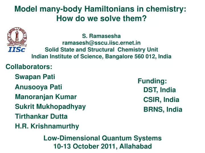
Model many-body Hamiltonians in chemistry: How do we solve them? S. Ramasesha ramasesh@sscu.iisc.ernet.in Solid State and Structural Chemistry Unit Indian Institute of Science, Bangalore 560 012, India Collaborators: Swapan Pati Anusooya Pati Manoranjan Kumar Sukrit Mukhopadhyay Tirthankar Dutta H.R. Krishnamurthy Funding: DST, India CSIR, India BRNS, India Low-Dimensional Quantum Systems 10-13 October 2011, Allahabad
o = S tij (aiaj+ H.c.) + S ai ni † i <ij> Theoretical Models for -Conjugated Systems Hückel Model: Carbon atoms are in sp2 hybridization. Assumes one pz orbital at every Carbon site involved in conjugation. Assumes transfer integral only between bonded Carbon sites. tij is resonance / transfer integral between bonded sites and ai, the site energy at site ‘i’.
(CH)x has charge conjugation or electron-hole or • alternancy symmetry. Carbon sites when subdivided • into two sublattices, no bonds between carbon atoms • on same sublattice. • The polymer also has inversion symmetry. • Weak spin-orbit interactions; states can be classified • by total spin. • Symmetries lead to strong experimental predictions. CA=CB CA=CB CA=CB CA=CB Symmetries in the MO picture
Alternancy Symmetry – Physicists’ View • Hamiltonian invariant for creation (annihilation) operators • replaced by annihilation (creation) operators such that • J a†A,i J† = bA,i and J a†B,i J† = -bB,i ; [H, J]=0 • Exists only if all sites are equivalent, transfer terms occur • only between ‘A’ sites and ‘B’ site. Valid at half-filling, for • diagonal interactions. • Requires system to be bipartite, transfer only between • sites on ‘A’ sublattice to sites on ‘B’ sublattice. • Known as electron-hole symmetry, charge conjugation • symmetry or bipartite system.
Consequences of Symmetry • Pairing theorem follows from alternancy symmetry • predicts that for ap bonding state at energy –ek, • there exists ap*anti-bondingstate at +ek. • Symmetry of states alternate between a+and b-, so • lowest energy excitation is dipole allowed. • Pairing theorem implies, (CH)x with odd number of carbon atoms should have a mid-gap state. • and a mid-gap absorption since lowest energy • excitation is dipole allowed.
+e1 +e1 b- b- +e2 +e2 a+ a+ +e3 +e3 b- b- +e4 +e4 a+ a+ Dipole allowed Dipole allowed e=0 e=0 Dipole allowed -e4 -e4 b- b- a+ a+ -e3 -e3 b- b- -e2 -e2 -e1 -e1 a+ a+ Schematic MO Picture of Even and Odd Polyenes Odd polyene Even polyene
C.B. Optical Gap Eg V.B. ( )x ( )y ( )x Polymer or Band Limit C.B. Dipole allowed Eg/2 Dipole allowed Eg/2 V.B. The kink in odd polyene is a topological soliton and is associated with a mid gap state.
Spin and Charge Solitons C.B. C.B. C.B. Eg/2 Eg/2 Eg/2 Eg/2 Eg Eg Eg V.B. V.B. V.B. - + ( ( )y ( ( )y ( ( )y )x )x )x Charged Soliton + ve Charged Soliton - ve Neutral soliton
Solitons, Polarons and Bipolarons C.B. C.B. C.B. Eg/2 V.B. V.B. V.B. Bipolaron Polaron Soliton Soliton has one sub-band gap transition. Polaron has three sub-band gap transition. Bipolaron has two sub-band gap transitions.
Experimental Status • Polyacetylene is a semiconductor due to Peierls’ • distortion. Valence band is filled and conduction * • band is empty. • The optical gap ~ 1.7eV. Dimerization required to obtain • this gap twice the observed bond length alternation. • Evidence for dipole forbidden states below Eg. • No evidence for mid-gap absorption in polyene radicals. • esr studies of polyene radicals show evidence for both • positive and negative spin densities.
R R C )X C SCD = + ( N N C R R PA Eg SCD 1/x Symmetric Cyanine Dyes: An intrigue SCD similar to (CH)x except for end groups. Qualitatively different Eg extrapolation in PA and SCD. Eg for Infinite chains in PA is nonzero, but in SCD it is zero.
Hückel model Single band for tight – binding molecules model in Solids Drawbacks of Hückel model: • Gives incorrect ordering of energy levels in polyenes. • Fails to account for negative spin densities in radicals and yields wrong spin-spin correlations. • Fails to reproduce qualitative differences between closely related systems. • Mainly of pedagogical value. Ignores explicit electron-electron interactions.
HFull = Ho + ½ Σ [ij|kl] (EijEkl – djkEil) ijkl Eij = S a†i,saj,s s Interacting p-Electron Models • Explicit electron – electron interactions essential for realistic modeling [ij|kl] = i*(1) j(1) (e2/r12) k*(2) l(2) d3r1d3r2 This model requires further simplification to enable routine solvability.
Zero Differential Overlap (ZDO) Approximation [ij|kl] = i*(1) j(1) (e2/r12) k*(2) l(2) d3r1d3r2 [ij|kl] = [ij|kl]ij kl
HHub = Ho + ΣUini(ni - 1)/2 i Hubbard Model • Hückel model + on-site repulsions [ii|jj] = 0 for i j ; [ii|jj] = Ui for i=j • Introduced in 1964. • Good for metals where screening lengths are short. • Half-filled one-band Hubbard model yields spin – 1/2 • antiferromagnetic Heisenberg model for U / t .
[ii|jj]parametrized byV( rij ) HPPP = HHub + Σ V(rij) (ni - zi) (nj - zj) i>j Pariser-Parr-Pople (PPP) Model • ziare local chemical potentials. • Ohno parametrization: • V(rij) = { [ 2 / ( Ui + Uj ) ]2 + rij2 }-1/2 • Mataga-Nishimoto parametrization: • V(rij) = { [ 2 / ( Ui + Uj ) ] + rij }-1
12 V13 HPPP = Σ tij (aiσajσ+ H.c.) + Σ(Ui /2)ni(ni-1) + Σ V(rij) (ni - 1) (nj - 1) † <ij>σ i i>j Model Hamiltonian PPP Hamiltonian (1953)
Exact Diagonalization (ED) Methods • Hilbert space of PPP Hamiltonian is finite for molecules. • PPP model conserves total S and MS. • Hilbert space factorized into definite total S and MS • spaces using Rumer-Pauling VB basis. • Rumer-Pauling VB basis is nonorthogonal, but complete, • and linearly independent. • Nonorthogonality of basis leads to nonsymmetric • Hamiltonian matrix • Formalism allows exploiting full spatial symmetry of any • point group.
Necessity and Drawbacks of ED Methods • ED methods are size consistent. Good for energy gap • extrapolations to thermodynamic or polymer limit. • Hilbert space dimension explodes with increase in • no. of orbitals • Nelectrons = 14, Nsites = 14, # of singlets = 2,760,615 • Nelectrons = 16, Nsites = 16, # of singlets = 34,763,300 • hence for polymers with large monomers (eg. PPV), ED • methods limited to small oligomers. • ED methods rely on extrapolations. In systems with large • p coherence length, ED methods may not be reliable. • ED methods provide excellent check on approximate • methods.
The Density Matrix Renormalization Group (DMRG) Technique • DMRG method involves iteratively building a large system • starting from a small system. • The eigenstate of superblock consisting of system and surroundings is used to build density matrix of system. • Dominant eigenstates (102 103) of the density matrix • are used to span the Fock space of the system. • The system size is increased by adding new sites. • Very accurate for one and quasi-one dimensional systems • such as Hubbard, Heisenberg spin chains and polymers S.R. White (1992)
Implementation of DMRG Method • Diagonalize a small system of say 4 sites with two on the left and two on the right ● ● ● ● {|L>} = {| >, | >, | >, | >} 1 2 2’ 1’ H = S1 S2 + S2 S2’ + S2’ S1’|yG> = S S CLR|L>|R> L R The summations run over the Fock space dimension L • Renormalization procedure for left block Construct density matrix rL,L’ = SRCLR CL’R Diagonalize density matrix r |ml > = ml |ml >, Construct renormalization matrix OL = [m1 m2· · · mm] is L x m; m < L • Repeat this for the right block
HL = OL HLOL† ; HL is the unrenormalized L x L left-block • Hamiltonian matrix, and HL is renormalized m x m • left-block Hamiltonian matrix. • Similarly, necessary matrices of site operator of left block • are renormalized. • The process is repeated for right-block operators with OR • The system is augmented by adding two new sites ● ● ● ● ● ● 1 2 3 3’ 2’ 1’ • The Hamiltonian of the augmented system is given by
Hamiltonian matrix elements in fixed DMEV Fock space • basis • Obtain desired eigenstate of augmented system • New left and right density matrices of the new eigenstate • New renormalized left and right block matrices • Add two new sites and continue iteration
Finite system DMRG If the goal is a system of 2N sites, density matrices employed enroute were those of smaller systems. The DMRG space constructed would not be the best This can be remedied by resorting to finite DMRG technique After reaching final system size, sweep through the system like a zipper While sweeping in any direction (left/right), increase corresponding block length by 1-site, and reduce the other block length by 1-site
Symmetrized DMRG Method Why do we need to exploit symmetries? • Important states in conjugated polymers: Ground state (11A+g); Lowest dipole excited state (11B-u); Lowest triplet state (13B+u); Lowest two-photon state (21A+g); mA+g state (large transition dipole to 11B-u); nB-u state (large transition dipole to mA+g) • In unsymmetrized methods, too many intruder states • between desired eigenstates. • In large correlated systems, only a few low-lying • states can be targeted; important states may • be missed altogether.
ai † = bi ; ‘i’ on sublattice A ai † = - bi ; ‘i’ on sublattice B Symmetries in the PPP and Hubbard Models Electron-hole symmetry: • When all sites are equivalent, for a bipartite system, electron-hole or charge conjugation or alternancy symmetry exists, at half-filling. • At half-filling the Hamiltonian is invariant under the • transformation
Eint. = 0, U, 2U,··· Covalent Space Even e-h space Includes covalent states Ne = N Eint. = 0, U, 2U,··· Dipole operator Eint. = U, 2U,··· Full Space Odd e-h space Excludes covalent states Ionic Space E-h symmetry divides N = Ne space into two subspaces: one containing both ‘covalent’ and ‘ionic’ configurations, other containing only ionic configurations. Dipole operator connects the two spaces.
Spin symmetries • Hamiltonian conserves total spin and z – component of total spin. • [H,S2] = 0 ; [H,Sz] = 0 • Exploiting invariance of the total Sz is trivial, but of the total S2 is hard. • When MStot. = 0, H is invariant when all the spins are rotated about the y-axis by p. This operation flips all the spins of a state and is called parity.
Stot. = 0,2,4, ··· Even parity space MS = 0 Stot. = 0,1,2, ··· Full Space Stot. =1,3,5, ··· Odd parity space Parity divides the total spin space into spaces of even total spin and odd total spin.
• The site e-h operator, Ji, has the property: • Ji|1> = |4> ; Ji|2> = h|2> ; Ji|3> =h |3> & Ji |4> = - |1> • h = +1 for ‘A’sublattice and –1 for ‘B’ sublattice • The site parity operator, Pi, has the property: • Pi |1> = |1> ; Pi |2> = |3> ; Pi |3> = |2> ; Pi |4> = - |4> Matrix Representation of Site e-h and Site Parity Operators in DMRG • Fock space of single site: • |1> = |0>; |2> = |>; |3> = |>; & |4> = |>
Matrix representation of system J and P • J of the system is given by • J = J1 J2 J3 ····· JN • P of the system is, similarly, given by • P = P1 P2 P3 ····· PN The overall electron-hole symmetry and parity matrices can be obtained as direct products of the individual site matrices. • Polymer also has end-to-end interchange symmetry C2 • The C2operation does not have a site representation
Symmetrized DMRG Procedure • At every iteration, J and P matrices of sub-blocks are renormalized to obtain JL, JR, PL and PR. • From renormalized JL, JR, PL and PR, thesuper block matrices, J and P are constructed. • Given DMRG basis states |m, s, s’, m’> • (|m> & |m’> are eigenvectors of density matrices, rL & rR • |s> & |s’> are Fock states of the two new sites) • super-block matrix J is given by Jm,s,s’,m’ ; n,t,t’,n’ = <m, s, s’, m’|J|n,t,t’,n’> = < m|JL|n> <s|J1|t> <s’|J1|t’> < m’|JR|n’>, • Similarly, the matrix P is obtained.
and from this, we can construct the matrix for C2. C2| m,s,s’,m’> = (-1)g | m’,s’,s,m>; g = (ns’ + nm’)(ns + nm) C2 Operation on the DMRG basis yields, J, P and C2 form an Abelian group Irr. representations,eA+, eA-, oA+, oA-, eB+, eB-, oB+, oB-; ‘e’ and ‘o’ imply even and odd under parity; ‘+’ and ‘-’ imply even and odd under e-h symmetry. Ground state lies in eA+, dipole allowed optical excitation in eB-, the lowest triplet in oB+.
1/h PG = S cG (R) R DG = 1/h S cG (R) cred. (R) R R Projection operator for an irreducible representation, G, PG , is The dimensionality of the space G is given by, Eliminate linearly dependent rows in the matrix of PG. Projection matrix S with DGrows and M columns. M is dimensionality of full DMRG space.
Symmetry operators JL, JR, PL, and PR for the augmented sub-blocks can be constructed and renormalized just as the other operators. • To compute properties, one could unsymmetrize the eigenstates and proceed as usual. • To implement finite DMRG scheme, C2 symmetry is used only at the end of each finite iteration. • Symmetrized DMRG Hamiltonian matrix, HS , is • given by, HS = SHS† H is Hamiltonian matrix in full DMRG space
DMRG Eg,N= 1.278, U/t =4 Eg,N= 2.895, U/t =6 DMRG Checks on SDMRG • Optical gap (Eg) in Hubbard model known analytically. In the limit of infinite chain length, for U/t = 4.0, Egexact= 1.2867 t ; U/t = 6.0 Egexact = 2. 8926 t PRB, 54, 7598 (1996).
The spin gap in the limit U/t should vanish for the Hubbard model. PRB, 54, 7598 (1996).
An Early Question in Organic Chemistry 1,3,5 Hexatriene unequal bond lengths Benzene equal bond lengths What will happen if the size (ring size or chain length) of the conjugated system is increased to infinity? • Peierls’ (1955) • System will be dimerized in the ground state
Uniform Cis Trans The case of polyacenes Is there a Peierls’ instability in polyacene? Is the ground state geometry Band structure of polyacenes corresponding to the three cases. Matrix element of symmetric perturbation between A and S band edges is zero. Conditional Peierls Instability. Bhargavi Srinivasan and S.R., Phys. Rev. B 57, 8927 (1998)
cis d =0.01 trans d =0.01 cis d =0.1 trans d =0.1 Role of Long-range Electron Correlations Used Pariser-Parr-Pople model within DMRG scheme Polyacene is built by adding two sites at a time.
DEA(N,d) = E(N,0) – E(N,d) ; A = cis / trans DEA(,d) = Lim. N {DEA(N,d) / N} For both cis and trans distortions, DEA(,d) d2 Peierls’ instability is conditional in polyacenes
d = 0 d = 0 Bond order – bond order correlations bi,i+1 = Ss (a†i,sai,s+ H.c.)
Exciton Binding Energy in Hubbard and U-V Models • We focus on lowest 11Bu exciton. • The conduction band edge Egis assumed to be corresponding to two long neutral chains giving well separated, freely moving positive and negative polarons • Exciton binding energy Eb is given by,