Download
1 / 13
130 likes | 208 Vues
Significance tests help accept or reject null hypothesis based on sampling distribution analysis. Learn how to use Chi-Square test to analyze the relationship between categorical variables with step-by-step examples. Gain insights into interpreting Chi-Square results and determining statistical significance.

E N D
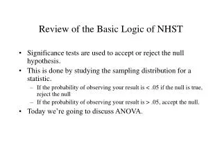
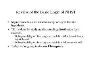
Review of the Basic Logic of NHST • Significance tests are used to accept or reject the null hypothesis. • This is done by studying the sampling distribution for a statistic. • If the probability of observing your result is < .05 if the null is true, reject the null • If the probability of observing your result is > .05, accept the null. • Today we’re going to discuss Chi-Square.
Chi-square • A common situation in psychology is when a researcher is interested in the relationship between two nominal or categorical variables. • The significance test used in this kind of situation is called a chi-square (2).
Chi-square example • We are interested in whether single men vs. women are more likely to own cats vs. dogs. • Notice that both variables are categorical. • Kind of pet: people are classified as owning cats or dogs (or both or neither). We can count the number of people belonging to each category; we don’t scale them along a dimension of pet ownership. • Sex: people are male or female. We count the number of people in each category; we don’t scale each person along a sex dimension.
Example Data • Males are more likely to have dogs as opposed to cats • Females are more likely to have cats than dogs NHST Question: Are these differences best accounted for by the null hypothesis or by the hypothesis that there is a real relationship between gender and pet ownership?
To answer this question, we need to know what we would expect to observe if the null hypothesis were true (i.e., that there is no relationship between these two variables, and any observed relationship is due to sampling error).
Example Data • To find expected value for a cell of the table, multiply the corresponding row total by the column total, and divide by the grand total • For the first cell (and all other cells), (50 x 50)/100 = 25 • Thus, if the two variables are unrelated, we would expect to observe 25 people in each cell
Example Data • The differences between these expected values and the observed values are aggregated according to the Chi-square formula:
NHST and chi-square • Once you have the chi-square statistic, it can be evaluated against a chi-square sampling distribution • The sampling distribution characterizes the range of chi-square values we might observe if the null hypothesis is true, but sampling error is giving rise to deviations from the expected values. • You can look up the probability value associated with a chi-square statistic in a table of using a computer • In our example in which the chi-square was 4.0, the associated p-value was >.05. (The chi-square statistic would have had to have been larger than 3.8 for it to have been significant.)
More complex situations • There may be more than two levels for any one variable. • Also, the base rates (i.e., the relative frequencies of the various subcategories) may be quite variable. • The logic and mechanics of the chi-square work the same way under these situations.
Another set of data • Here we have the same variables, but the base rate of dog lovers is much higher (e.g., the column totals indicate that, regardless of sex, 80 of 100 people own dogs) • We procede as we did before
Observed Frequencies Expected Frequencies 25 is larger than 3.8, so p <.05
Another set of data • Now one of our variables has 3 subcategories or levels instead of two.
Observed Frequencies Expected Frequencies Chi-square would need to be greater than 5.9 for p < .05.