Download
1 / 38
550 likes | 1.43k Vues
The stability of the solar system. TexPoint fonts used in EMF. Read the TexPoint manual before you delete this box.: A A A A A A A A A A. Stability of the solar system. The problem:

E N D
The stability of the solar system TexPoint fonts used in EMF. Read the TexPoint manual before you delete this box.: AAAAAAAAAA
Stability of the solar system The problem: A point mass is surrounded by N > 1 much smaller masses on nearly circular, nearly coplanar orbits. Is the configuration stable over very long times (up to 1010 orbits)? Why is this interesting? • one of the oldest problems in theoretical physics • what is the fate of the Earth? • why are there so few planets in the solar system? • can we calibrate geological timescale over the last 50 Myr? • how do dynamical systems behave over very long times? • can we explain the properties of extrasolar planetary systems?
Stability of the solar system Newton: “blind fate could never make all the Planets move one and the same way in Orbs concentric, some inconsiderable irregularities excepted, which could have arisen from the mutual Actions of Planets upon one another, and which will be apt to increase, until this System wants a reformation” Laplace: “An intelligence knowing, at a given instant of time, all forces acting in nature, as well as the momentary positions of all things of which the universe consists, would be able to comprehend the motions of the largest bodies of the world and those of the smallest atoms in one single formula, provided it were sufficiently powerful to subject all data to analysis. To it, nothing would be uncertain; both future and past would be present before its eyes.”
Stability of the solar system The problem: A point mass is surrounded by N much smaller masses on nearly circular, nearly coplanar orbits. Is the configuration stable over very long times (up to 1010 orbits)? How can we solve this? • many famous mathematicians and physicists have attempted to find solutions, with limited success (Newton, Laplace, Lagrange, Gauss, Poincaré, Kolmogorov, Arnold, Moser, etc.) • only feasible approach is numerical solution of equations of motion by computer, but: • needs 1012 timesteps so lots of CPU • needs sophisticated algorithms to avoid buildup of errors • inherently serial so little gain from massively parallel computers
2 ( ) N ¡ d x x m P j i j x l l G i i t ¡ + s m a c o r r e c o n s = 2 j j 3 j 1 d t ¡ = x x i j Stability of the solar system “Small corrections” include: • general relativity (fractional effect <10-8) • satellites (<10-7) Unknowns include: • asteroids (< 10-9) and Kuiper belt (< 10-6 even for outermost planets) • solar quadrupole moment (< 10-10) • mass loss from Sun through radiation and solar wind, and drag of solar wind on planetary magnetospheres (< 10-14) • Galactic tidal forces (fractional effect < 10-13) • passing stars (closest passage about 500 AU) Masses mj known to better than 10-9M Initial conditions known to fractional accuracy better than 10-7 1 AU = 1 astronomical unit = Earth-Sun distance Neptune orbits at 30 AU solar mass
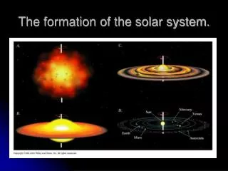
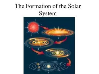
Stability of the solar system To a very good approximation, the solar system is an isolated, conservative dynamical system described by a known set of equations, with known initial conditions All we have to do is integrate the equations of motion for ~1010 orbits (4.5109 yr backwards to formation, or 7109 yr forwards to red-giant stage when Mercury and Venus are swallowed up) Goal is quantitative accuracy ( 1 radian) over 108 yr and qualitative accuracy over 1010 yr
A primer on orbit integration Consider integrating an orbit in the Kepler potential V(r) = -1/r. Equations of motion for particle of unit mass read Examine three integration methods with timestep h: Euler’s method Modified Euler method Runge-Kutta method Error after integrating for unit time is O(h) for Euler methods and O(h4) for Runge-Kutta (first-order versus fourth-order) 100 function evaluations per orbit for each method
A primer on orbit integration Modified Euler method comes in two flavors: “drift-kick” “kick-drift” An even better method is to combine half a drift-kick step and half a kick-drift step: This is the classic leapfrog or Verlet method.
A primer on orbit integration Why does modified Euler work so well? Because it: • preserves volume in phase space, just like Newton’s laws (Liouville’s theorem): • generates a symplectic or canonical transformation Modified Euler method is the prototype of geometric integration algorithms Why does leapfrog work even better than modified Euler? Because: • like modified Euler, it generates a symplectic transformation • it has error O(h2), one order higher than modified Euler • is time-reversible, just like Newton’s laws (a second geometric property)
A primer on orbit integration The system we are examining is described by the Hamiltonian and the equations of motion Any map r(0), p(0) r(t), p(t) generated by a Hamiltonian is a canonical or symplectic transformation. So consider Integrating this from t=0+ to t=h+ gives which is the modified Euler method. Leapfrog is simply
A primer on orbit integration To follow motion in the potential V(r) we use the Hamiltonian Motion of a test particle in a planetary system is described by the Hamiltonian To carry out numerical integration we replace this with
A primer on orbit integration The workhorse for long orbit integrations is the mixed-variable symplectic integrator (Wisdom & Holman 1991) a geometric integrator (symplectic and time-reversible) errors smaller than leapfrog by of order mplanet/M* 10-4 all of the work is in converting back and forth from action-angle variables to Cartesian coordinates once per step numerical analysis dynamical perturbation theory long-term errors reduced to O(mplanet/M*)2 by techniques such as warmup
A primer on roundoff error Roundoff error can cause big problems: • in 1991 Gulf War, Patriot missile defense system converted clock steps of 0.1 sec to decimal by multiplying by a 22-bit binary number; after 100 hours the accumulated roundoff error was 0.3 sec, which led to failure to intercept a Scud missile, resulting in 28 deaths Floating-point numbers are stored in the computer as pbits plus an exponent. Typically p=53, corresponding to accuracy =2-p'10-16 Simplest model is that energy error grows like a random walk. After N integration steps the fractional error is E/E N1/2 t1/2. Phase error is then (t/Porbit) E/E t3/2(“good” roundoff) Many numerical integrations exhibit t2 (“bad” roundoff”) Over lifetime of solar system, 1 for good roundoff and 105 radians for bad roundoff
A primer on roundoff error Most important step in managing roundoff is to ensure “good” roundoff behavior rather than “bad” behavior. To manage roundoff error: • use machines with optimal and unbiased arithmetic, e.g., IEEE 754 standard (to check it out, use “paranoia” programs at www.netlib.org) • carry out selected operations in extended or quadruple precision • beware of any mathematical constants that are not representable (, 1/3, etc.). Replace (2.0/3.0)*x by 2.0*x/3.0
A primer on orbit integration Lessons: • when integrating ordinary differential equations, short-term quantitative accuracy is not the same as---and is often less important than---long-term qualitativeaccuracy • use geometric integrators, which preserve the qualitative features of the physical systems they are describing (symplecticity, time-reversibility, energy and angular momentum conservation, flux conservation, unitarity, etc.) • if the physical system is close to one that can be integrated exactly, choose the integration algorithm so that it is exact for the integrable system • Hamiltonian mechanics is actually useful
0 - 55 Myr +4.5 Gyr • an integration of the solar system (Sun + 9 planets) for § 4.5£ 109 yr=4.5 Gyr • figures show innermost four planets Ito & Tanikawa (2002) -55 – 0 Myr -4.5 Gyr
Pluto’s peculiar orbit Pluto has: • the highest eccentricity of any planet (e = 0.250 ) • the highest inclination of any planet ( i = 17o ) • closest approach to Sun is q = a(1 – e) = 29.6 AU, which is smaller than Neptune’s semimajor axis ( a = 30.1 AU ) How do they avoid colliding?
Pluto’s peculiar orbit Orbital period of Pluto = 247.7 y Orbital period of Neptune = 164.8 y 247.7/164.8 = 1.50 = 3/2 Resonance ensures that when Pluto is at perihelion it is approximately 90o away from Neptune Resonant argument: • 3(longitude of Pluto) 2(longitude of Neptune) – (perihelion of Pluto) librates around with 20,000 year period (Cohen & Hubbard 1965)
Pluto’s peculiar orbit PPluto/PNeptune early in the history of the solar system there was debris left over between the planets ejection of this debris by Neptune caused its orbit to migrate outwards if Pluto were initially in a low-eccentricity, low-inclination orbit outside Neptune it is inevitably captured into 3:2 resonance with Neptune once Pluto is captured its eccentricity and inclination grow as Neptune continues to migrate outwards other objects may be captured in the resonance as well Pluto’s semi-major axis Pluto’s eccentricity Pluto’s inclination resonant argument Malhotra (1993)
Kuiper belt objects Plutinos (3:2) Centaurs comets from Minor Planet Center
Regular highly predictable, “well-behaved” small differences in position and velocity grow linearly: x, v t e.g. baseball, golf, simple pendulum, all problems in mechanics textbooks, planetary orbits on short timescales Chaotic difficult to predict, “erratic” small differences grow exponentially at large times: x, v exp(t/tL) where tL is Liapunov time appears regular on timescales short compared to Liapunov time linear growth on short times, exponential growth on long times e.g. roulette, dice, pinball, weather, billiards Two kinds of dynamical system
exponential, exp(t/tL) separation in phase space linear, t 10 Myr Laskar (1989)
saturated factor of 1000 factor of 10,000 Jupiter Pluto 400 million years 300 million years The orbit of every planet in the solar system is chaotic (Sussman & Wisdom 1988, 1992) separation of adjacent orbits grows exp(t / tL) where Liapunov time tL is 5-20 Myr factor of at least 10100 over lifetime of solar system
saturated Hayes (astro-ph/0702179) Liapunov time tL=12 Myr Integrators: • double-precision (p=53 bits) 2nd order mixed-variable symplectic (Wisdom-Holman) method with h=4 days and h=8 days • double-precision (p=53 bits) 14th order multistep method with h=4 days • extended-precision (p=80 bits) 27th order Taylor series method with h=220 days 200 Myr
Chaos in the solar system • orbits of inner planets (Mercury, Venus, Earth, Mars) are chaotic with e-folding times for growth of small changes (Liapunov times) of 5-20 Myr (i.e. 200-1000 e-folds in lifetime of solar system • chaos in orbits of outer planets depends sensitively on initial conditions but usually are chaotic • positions (orbital phases) of planets are not predictable on timescales longer than 100 Myr – future of solar system over longer times can only be predicted probabilistically • the solar system is a poor example of a deterministic universe • shapes of some orbits execute random walk on timescales of Gyr or longer
Laskar (1994) start finish
Causes of chaos • dynamical behavior of non-linear systems is largely determined by resonance structure • a resonance of strength ² in linear theory has an effective width in phase space »²1/2 • chaos in non-linear systems arises from overlap of resonances • orbits with 3 degrees of freedom have three fundamental frequencies i. In spherical potentials, 1=0. In Kepler potentials 1=2=0 so resonances are strongly degenerate • planetary perturbations lead to fine-structure splitting of resonances by amount O() where mplanet/M*. • two-body resonances have strength O() and width O()1/2 so width of each resonance is much larger than width of multiplet • more numerous three-body resonances have strength O(2) and width O(). • Murray & Holman (1999) show that chaos in outer solar system arises from overlap in the multiplet of 3-body resonance with critical argument = 3(longitude of Jupiter) - 5(longitude of Saturn) - 7(longitude of Uranus) • small changes in initial conditions can eliminate or enhance chaos • cannot predict lifetimes analytically
Consequences of chaos • orbits of inner planets (Mercury, Venus, Earth, Mars) are chaotic with e-folding times for growth of small changes (Liapunov times) of 5-20 Myr (i.e. 200-1000 e-folds in lifetime of solar system • chaos in orbits of outer planets depends sensitively on initial conditions but usually are chaotic • positions (orbital phases) of planets are not predictable on timescales longer than 100 Myr • the solar system is a poor example of a deterministic universe • shapes of some orbits execute random walk on timescales of Gyr or longer • most chaotic systems with many degrees of freedom are unstable because chaotic regions in phase space are connected so trajectory wanders chaotically through large distances in phase space (“Arnold diffusion”). Thus solar system is unstable, although probably on very long timescales • most likely ejection has already happened one or more times
J S U N age of solar system Holman (1997)
Summary • we can integrate the solar system for its lifetime • the solar system is not boring on long timescales • planet orbits are probably chaotic with e-folding times of 5-20 Myr • the orbital phases of the planets are not predictable over timescales > 100 Myr • “Is the solar system stable?” can only be answered probabilistically • it is unlikely that any planets will be ejected or collide before the Sun dies • most of the solar system is “full”, and it is likely that planets have been lost from the solar system in the past
Sunday, January 13, 14:30, Lewiner seminar room • New worlds: the properties and evolution of extrasolar planetary systems • Monday, January 14, 16:30, Lidow 502 • Kozai oscillations in binary stars and planetary systems
Bode’s law planets suffer no close encounters and are spaced fairly regularly (Bode’s law: an=0.4 + 0.32n) *predicted +exceptions
Brown et al. (2005) • diameter 2400 § 100 km or 5% bigger than Pluto • has a moon • albedo 80-90%