Download
1 / 14
251 likes | 1.14k Vues
Molecular Speeds. Maxwell-Boltzmann Distribution Physical interpretation According to this, if the temperature drops from 20°C to -20°C, v p changes by 7%.

E N D
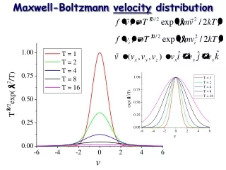
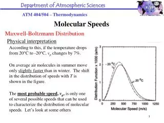
Molecular Speeds Maxwell-Boltzmann Distribution Physical interpretation According to this, if the temperature drops from 20°C to -20°C, vp changes by 7%. On average air molecules in summer move only slightly faster than in winter. The shift in the distribution of speeds with T is shown in the figure. The most probable speed, vp, is only one of several possible speeds that can be used to characterize the distribution of molecular speeds. Let’s look at some others
Molecular Speeds Maxwell-Boltzmann Distribution Physical interpretation The mean speedis written as The root-mean-square speedis written as Where The three speeds are shown on the right. They are not all that different (ratio 1:1.13:1.22). Any one of them could be used to specify the average speed, you just need to specify which average you use.
Intermolecular Separation • Characteristic of gas – mostly empty space • From the ideal gas law where n is the number density (#/m3) of molecules. • Inverse of n is the average volume of space allocated to each molecule. Then where d is the average separation between molecules.
Intermolecular Separation • Take p = 105 Pa, and T = 293 K • We calculate d = 3.43 × 10⁻⁹ m (3.43 nm) • While molecules have no sharp boundaries, the approximate diameter of common atmospheric molecules is d0= 0.3 nm. • Volume fraction of air occupied by matter is the ratio of the molecular volume to the volume allocated to the molecule, i.e., (d0/d)3 10-3. About 1 part per 1000 (by volume) of air is occupied by matter.
Mean Free Path • Intermolecular separation “d” is not the distance a molecule must travel before interacting with another. • Consider cylindrical volume of cross section A, length x, and molecular number density n ( 3 × 1019 cm-3), then the total number of molecules is N = nAx. • Assume molecules are spheres of diameter, d0. • Two spheres interact when centers approach each other within d0. • Consider projectile molecule a point and target molecule as sphere with collision cross section = d02. • 3 × 10-15 cm2
Mean Free Path • Consider a point molecule incident at one end of the cylinder traveling parallel to cylinder x-axis. Its position on A where it enters the cylinder is random. • Question: How far will it go before it collides with a target molecule? • Some may travel a short distance and some a longer distance. • The target area presented to point molecule over distance xis nAx. • Total target cross-sectional area per cylinder cross sectional area is nx. • This is, approximately, the probability that a point molecule will have a collision in distancex.
Mean Free Path • If nx = 1, the molecule is unlikely to not collide. • Corresponding distance, x = , at which n = 1 is the mean free path. • As n increases, decreases. • As decreases, increases. • Because number density n decreases exponentially with z, increases exponentially. • A more exact derivation would lead to the same expression, but with a numerical constant that is close to 1.
Mean Free Path • Example: Using = 3 × 10-15 cm2, and n = 3 × 1019 cm-3, we get a mean free path of ~0.1 m, ~an order of magnitude+ greater (30 times greater) than the average molecular separation (~3.4 nm). • Result makes physical sense. • In order for d, after each collision the molecule would have to rebound at an angle exactly toward its nearest neighbor. Not likely.
Intermolecular Collision Rate • Assume all molecules are fixed, except one. • All fixed molecules are points, the moving molecule a sphere with projected area . • In time Δtthe molecule moving at speed v sweeps out a volume vΔt. • All fixed molecules collide with moving molecule. • Total number of collisions in time Δt is nvΔt.
Intermolecular Collision Rate • Collision rate obtained by dividing by Δt. • This yields nv, the collision rate per molecule. • To obtain the collision rate per unit volume, multiply by the number density of molecules, n. • This yields the volume collision rate n2v. • Because molecules are distributed in speed, we should interpret v as a mean relative speed. • We know that mean speeds are proportional to T ½. • Using this result and the ideal gas law, we can write the rate of intermolecular collisions/unit volume in a gas in the form shown, where C is a constant of order 1:
Intermolecular Collision Rate • Example: Consider 2 different gases, both at the same T and p, but with different collision cross sections and masses. • According to our result, the intermolecular collision rates are different because m and are different. • This tells us that neither p nor T is determined by intermolecular collision rates. • None of the thermodynamic variables (p, T, ) depends explicitly on collisions. Collisions provide for energy and momentum transfer, however (randomization). • For n = 1019 cm-3, = 10-15 cm2, and v = 400 m/s, the collision rate = 4 × 1027 cm-3 s-1!! This high collision rate is at the heart of the local thermodynamic equilibrium.