Non-Conservative Boltzmann equations Maxwell type models
710 likes | 897 Vues
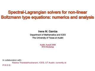
Non-Conservative Boltzmann equations Maxwell type models. Irene Martinez Gamba Department of Mathematics and ICES The University of Texas at Austin. Buenos Aires, Diciembre 06. In collaboration with: A. Bobylev, Karlstad Univesity, Sweden C. Cercignani, Politecnico di Milano, Italy.

Non-Conservative Boltzmann equations Maxwell type models
E N D
Presentation Transcript
Non-Conservative Boltzmann equationsMaxwell type models Irene Martinez Gamba Department of Mathematics and ICES The University of Texas at Austin Buenos Aires, Diciembre 06 In collaboration with: A. Bobylev, Karlstad Univesity, Sweden C. Cercignani, Politecnico di Milano, Italy.
The Boltzmann Transport Equation (BTE) is a model from an statistical description of a flow of ``particles'' moving and colliding or interacting in a describable way ‘by a law’; and the average free flight time between stochastic interactions (mean free path Є) inversely proportional to the collision frequency. • Example: Think of a `gas': particles are flowing moving around “billiard-like” interacting into each other in such setting that • The particles are so tightly pack that only a few average quantities will • described the flow so,Є<< 1(macroscopic or continuous mechanical system) • There are such a few particles or few interactions that you need a complete description of each particle trajectory soЄ>> 1,(microscopic or dynamical systems), • There are enough particles in the flow domain to have “good” statistical assumptions such that Є =O(1)(Boltzmann-Grad limit): • mesoscopic or statistical models and systems.
Examples are Non-Equilibrium Statistical States (NESS) in N dimensions, Variable Hard Potentials (VHP , 0<λ ≤1) and Maxwell type potentials interactions (λ=0). • Rarefied ideal gases-elastic (conservative) classical theory, • Gas of elastic or inelastic interacting systems in the presence of a thermostat with a fixed background temperature өb or Rapid granular flow dynamics: (inelastic hard sphere interactions): homogeneous cooling states, randomly heated states, shear flows, shockwaves past wedges, etc. • Bose-Einstein condensates models and charge transport in solids: current/voltage transport modeling semiconductor nano-devices. • Emerging applications from Stochastic dynamics for multi-linear Maxwell type interactions : Multiplicatively Interactive Stochastic Processes: • Pareto tails for wealth distribution, non-conservative dynamics: opinion dynamic models, particle swarms in population dynamics, etc (Fujihara, Ohtsuki, Yamamoto’ 06,Toscani, Pareschi, Caceres 05-06…). • Goals: • Understanding of analytical properties: large energy tails • long time asymptotics and characterization of asymptotics states • A unified approach for Maxwell type interactions.
u’= |u| ω and u . ω= cos(ө) |u| Notice: ω direction of specular reflection =σ
α < 1 loss of translational component for u but conservation of the rotational component of u
In addition: Classical n-D-Boltzmann equation formulation for binary elastic or inelastic collisions for VHP or Maxwell interactions, in the (possible) presence of ‘heating sources’ or dynamical rescaling
The Boltzmann Theorem:there are only N+2 collision invariants
Molecular models of Maxwell type Bobylev, ’75-80, for the elastic, energy conservative case-Bobylev, Cercignani, I.M.G’06, for general non-conservative problem
Where, for the Fourier Transform of f(t,v) in v: The transformed collisional operator satisfies, by symmetrization in v and v* with Since then For
Typical Spectral function μ(p) for Maxwell type models Self similar asymptotics for: • For p0 >1 and 0<p< (p +Є) < p0 For any initial state φ(x) = 1 – xp + x(p+Є) , p ≤ 1. Decay rates in Fourier space: (p+Є)[ μ(p) - μ(p +Є) ] For finite (p=1) or infinite (p<1) initial energy. μ(p) For μ(1) = μ(s*), s* >p0 >1 Power tails Kintchine type CLT p0 s* 1 μ(s*)=μ(1) μ(po) No self-similar asymptotics with finite energy • For p0< 1 and p=1