Download

1 / 26
260 likes | 281 Vues
Learn how to test if data distribution fits a claimed distribution using chi-square. Explore Multinomial Experiments and practical examples.

E N D
Section 11-1 & 11-2 Overview and Chi-Square Goodness of Fit Test
We focus on analysis of categorical(qualitative or attribute) data that can be separated into different categories(often called cells). • Use the 2 (chi-square) test statistic (Table A-4). • The goodness-of-fit test uses a one-way frequency table (single row or column). Analyzing Categorical Data
Purpose of the Goodness of Fit Test Given data separated into different categories, we will test the hypothesis that the distribution of the data agrees with or “fits” some claimed distribution. The hypothesis test will use the chi-square distribution with the observed frequency counts and the frequency counts that we would expect with the claimed distribution.
Multinomial Experiment This is an experiment that meets the following conditions: 1. The number of trials is fixed. 2. The trials are independent. 3. All outcomes of each trial must be classified into exactly one of several different categories. 4. The probabilities for the different categories remain constant for each trial.
A goodness-of-fit test is used to test the hypothesis that an observed frequency distribution fits (or conforms to) some claimed distribution. Goodness-of-fit Test
Orepresents the observed frequency of an outcome. Erepresents the expected frequency of an outcome. krepresents the number of different categories or outcomes. nrepresents the total number of trials. Goodness-of-Fit Test Notation
n E = k If all expected frequencies are equal: the sum of all observed frequencies divided by the number of categories Expected Frequencies
If expected frequencies are not all equal: Each expected frequency is found by multiplying the sum of all observed frequencies by the probability for the category. E = np Expected Frequencies
The data have been randomly selected. • The sample data consist of frequency counts for each of the different categories. • For each category, the expected frequency is at least 5. (The expected frequency for a category is the frequency that would occur if the data actually have the distribution that is being claimed. There is no requirement that the observed frequency for each category must be at least 5.) Goodness-of-Fit Test in Multinomial Experiments: Requirements/Assumptions
2= (O – E)2 E Critical Values 1. Found in Table A-4 using k – 1 degrees of freedom, where k =number of categories. 2. Goodness-of-fit hypothesis tests are always right-tailed. TestStatistic Goodness-of-Fit Test in Multinomial Experiments
A large disagreement between observed and expected values will lead to a large value of 2and a small P-value. • A significantly large value of 2 will cause a rejection of the null hypothesis of no difference between the observed and the expected. • A close agreement between observed and expected values will lead to a small value of 2 and a large P-value. Goodness-of-Fit Test in Multinomial Experiments
Relationships Among the 2 Test Statistic, P-Value, and Goodness-of-Fit Figure 11-3
Example: Last Digits of Weights When asked, people often provide weights that are somewhat lower than their actual weights. So how can researchers verify that weights were obtained through actual measurements instead of asking subjects?
Example: Last Digits of Weights Test the claim that the digits in Table 11-2 do not occur with the same frequency. Table 11-2 summarizes the last digit of weights of 80 randomly selected students.
Example: Last Digits of Weights Verify that the assumptions for the Hypothesis test have been met. 1. Assume a random sample of student weights. 2. Expected counts are 8 for every category which is greater than 5 therefore, the sample is large enough.
Example: Last Digit Analysis Test the claim that the digits in Table 11-2 do not occur with the same frequency. H0: p0 = p1 = = p9 H1: At least one of the probabilities is different from the others. = 0.05 k – 1 = 9 2 critical value= 16.919
Example: Last Digit Analysis Test the claim that the digits in Table 11-2 do not occur with the same frequency. Because the 80 digits would be uniformly distributed through the 10 categories, each expected frequency should be 8.
Example: Last Digit Analysis Test the claim that the digits in Table 11-2 do not occur with the same frequency.
Example: Last Digit Analysis Test the claim that the digits in Table 11-2 do not occur with the same frequency. From Table 11-3, the test statistic is 2 = 156.500. Since the critical value is 16.919, we reject the null hypothesis of equal probabilities. There is sufficient evidence to support the claim that the last digits do not occur with the same relative frequency.
Example: Detecting Fraud Unequal Expected Frequencies In the Chapter Problem, it was noted that statistics can be used to detect fraud. Table 11-1 lists the percentages for leading digits from Benford’s Law.
Example: Detecting Fraud Unequal Expected Frequencies In the Chapter Problem, it was noted that statistics can be used to detect fraud. Table 11-1 lists the percentages for leading digits from Benford’s Law.
Observed Frequencies and Frequencies Expected with Benford’s Law Example: Detecting Fraud Test the claim that there is a significant discrepancy between the leading digits expected from Benford’s Law and the leading digits from the 784 checks.
Example: Detecting Fraud Test the claim that there is a significant discrepancy between the leading digits expected from Benford’s Law and the leading digits from the 784 checks. H0: p1 = 0.301, p2 = 0.176, p3 = 0.125, p4 = 0.097, p5 = 0.079, p6 = 0.067, p7 = 0.058, p8 = 0.051 and p9 = 0.046 H1: At least one of the proportions is different from the claimed values. = 0.01 k – 1 = 8 2.01,8 = 20.090
Example: Detecting Fraud Test the claim that there is a significant discrepancy between the leading digits expected from Benford’s Law and the leading digits from the 784 checks. The test statistic is 2 = 3650.251. Since the critical value is 20.090, we reject the null hypothesis. There is sufficient evidence to reject the null hypothesis. At least one of the proportions is different than expected.
Example: Detecting Fraud Test the claim that there is a significant discrepancy between the leading digits expected from Benford’s Law and the leading digits from the 784 checks. Figure 11-5
Example: Detecting Fraud Figure 11-6 Comparison of Observed Frequencies and Frequencies Expected with Benford’s Law