Download
1 / 48
490 likes | 900 Vues
Nonparametric tests, rank-based tests, chi-square tests. Parametric tests. Parameter: a parameter is a number characterizing an aspect of a population (such as the mean of some variable for the population), or that characterizes a theoretical distribution shape.

E N D
Parametric tests • Parameter: a parameter is a number characterizing an aspect of a population (such as the mean of some variable for the population), or that characterizes a theoretical distribution shape. • Usually, population parameters cannot be known exactly; in many cases we make assumptions about them. • Parameters of the normal distribution: , • Parameter of the binomial distribution: n, p • Parameter of the Poisson distribution:
Parametric tests • The null hypothesis contains a parameter of a distribution. The assumptions of the tests are that the samples are drawn from a normally distributed population. So t-tests are parametric tests. • One sample t-test: H0: =c, • Two sample t-test: H0: 1=2,assumptions: 12=22
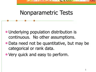
Nonparametric tests • We do not need to make specific assumptions about the distribution of data. • They can be used when • The distribution is not normal • The shape of the distribution is not evident • Data are measured on an ordinal scale (low-normal-high, passed – acceptable – good – very good)
Ranking data • Nonparametric tests can't use the estimations of population parameters. They use ranks instead. Instead of the original sample data we have to use its rank. • To show the ranking procedure suppose we have the following sample of measurements: 199, 126, 81, 68, 112, 112. • Sort the data in ascending order: 68, 81,112,112,126,199 • Give ranks from 1 to n: 1, 2, 3, 4, 5, 6 • Two cases are equal, they are assigned a rank of 3.5, the average rank of 3 and 4. We say that case 5 and 6 are tied. • Ranks corrected for ties: 1, 2, 3.5, 3.5, 5, 6
Case Data Rank Ranks corrected for ties 4 68 1 1 3 81 2 2 5 112 3 3.5 6 112 4 3.5 2 126 5 5 1 199 6 6 The sum of all ranks must be Using this formula we can check our computations. Now the sum of ranks is 21, and 6(7)/2=21. Result of ranking data
Nonparametric tests for paired data(nonparametric alternatives of paired t-test) • Sign test • Wilcoxon’s matched pairs test • Null hypothesis: the paired samples are drawn from the same population
Nonparametric test for data in two independent groups(nonparametric alternatives of two sample t-test) • Mann-Whitney U test • Null hypothesis: the samples are drawn from the same population • Assumption: the distribution of variables is continuous and the density functions have the same shape
Nonparametric alternative of the correlation coefficient : Spearman's rank correlation coefficient. • The rank correlation coefficient rs one of the nonparametric measure of statistical dependence. It is the Pearson’s correlation coefficient based on the ranks of the data if there are no ties (adjustments are made if some of the data are tied). • –1≤ rs ≤+1 • Its significance can be tested using the same formula as in testing the Pearson’s coefficient of correlation.
Chi-square tests Nonparametric tests but they are not based on ranks
Example • A study was carried out to investigate the proportion of persons getting influenza vary according to the type of vaccine. Given below is a 3 x 2 table of observed frequencies showing the number of persons who did or did not get influenza after inoculation with one of three vaccines. • Does proportion of getting influenza depend on the type of vaccine?
Test of independence • In biology the most common application for chi-squared is in comparing observed counts of particular cases to the expected counts. • A total of n experiments may have been performed whose results are characterized by the values of two random variable X and Y. • We assume that the variables are discrete and the values of X and Y are x1, x2,...,xr and y1, y2,...,ys, respectively, which are the outcomes of the events A1,A2,...,Ar and B1, B2,...,Bs . Let's denote by kij the number of the outcomes of the event (Ai, Bj). These numbers can be grouped into a matrix, called a contingency table. It has the following form:
Contingency table Frequency of Aievent i=1,2,…r Frequency of Bievent j=1,2,…s
Chi-square test (Pearson) • H0: The two variables are independent. Mathematically: P(AiBj) = P (Ai) P( Bj ) • Test statistic: • If H0 is true, then 2 has asymptotically 2 distribution with (r-1)(s-1) degrees of freedom. • Decision: if 2 > 2table then we reject the null hypothesis that the two variables are independent, in the opposite case we do not reject the null hypothesis.
Observed (Oij)= kij Expected (Eij)=: Row total*column total/n Observed and expected frequencies
Example • A study was carried out to investigate the proportion of persons getting influenza vary according to the type of vaccine. Given below is a 3 x 2 table of observed frequencies showing the number of persons who did or did not get influenza after inoculation with one of three vaccines. • There are two categorical variables (type of vaccine, getting influenza) • H0: The two variables are independent • proportions getting influenza are the same for each vaccine
Calculation of the test statistic Observed frequencies Expected frequencies • ²=13.6 • Degrees of freedom: {(r–1 )(c–1 )=} (2-1)*(3-1)=2 • Here 2 =13.6> 2table =5.991;(df=2;α=0.05). We reject the null hypothesis • We conclude that the proportions getting influenza are not the same for each type of vaccine
Assumption of the chi-square test • Expected frequencies should be big enough • The number of cells with expected frequencies < 5 can be maximum 20% of the cells. • For example, in case of 6 cells, expected frequencies <5 can be in maximum 1 cell (20% of 6 is 1.2)
SPSS results • a. Assumption for expected frequencies are OK • ²=13.06 and p=0.001 • Here p=0.001 < α=0.05 we reject the null hypothesis. • We conclude that the proportions getting influenza are not the same for each type of vaccine
The square contingency table Testing for independence
Chi-square test for 2x2 tables • Formula of the test statistic • Frank Yates, an English statistician, suggested a correction for continuity that adjusts the formula for Pearson's chi-square test by subtracting 0.5 from the difference between each observed value and its expected value in a 2 × 2 contingency table. This reduces the chi-square value obtained and thus increases its p-value.
Example • We are going to compare the proportions of two different treatments’ output. Our data are tabulated below. • H0: the outcome is independent of treatment in the population.
Solution based on obseved and expected frequencies Observed Expected
Decision • Here Pearson 2 =0.796 <2table =3.841 thus we accept the null hypothesis that the two variables are independent • SPSS p-value (=0.372) is greater than α=0.05 so thus we accept also the null hypothesis that the two variables are independent
Notes • Both variables are dichotomous • The Chi-squares give only an estimate of the true Chi-square and associated probability value, an estimate which might not be very good in the case of the marginals being very uneven or with a small value (~less than five) in one of the cells • In that case the Fisher Exact is a good alternative for the Chi-square. However, with a large number of cases the Chi-square is preferred as the Fisher is difficult to calculate.
Fisher’s-exact test Calculation of the p-value is based on the permutational distribution of the test Statistic (without using chi-square formula).
Fisher-exact test • The procedure, ascribed to Sir Ronald Fisher, works by first using probability theory to calculate the probability of observed table, given fixed marginal totals. • Note: n factorial: n!=123…n, 0!=1
Observed probabilities Original table Possible re-arrangements Fisher’s p-value=0,119+0,0476=0,167 Fisher showed that to generate a significance level, we need consider only the cases where the marginal totals are the same as in the observed table, and among those, only the cases where the arrangement is as extreme as the observed arrangement, or more so.
The chi-square test for goodness of fit • Goodness of fit tests are used to determine whether sample observation fall into categories in the way they "should" according to some ideal model. When they come out as expected, we say that the data fit the model. The chi-square statistic helps us to decide whether the fit of the data to the model is good. • H0: the distribution of the variable X is a given distribution
Categorical variable. Example. A dice is thrown 120 times. We would like to test whether the dice is fair or biased. Observed frequencies Continuous variable Example. We would like to test whether the sample is drawn from a normally distributed population.Distribution of ages The distribution of the sample depending on the type of the variable
Suppose we have a sample of n observations. Let's prepare a bar chart or a histogram of the sample – depending on the type of the variable. In both cases, we have frequencies of categories or frequencies in the interval. • Let's denote the frequency in the i-th category or interval by ki, i=1,2,…,r (r is the number of categories). • Let's denote pi the probabilities of falling into a given category or interval in the case of the given distribution. • If H0 is true and n is large, then the relative frequencies are approximations of pi -s, or . • The formula of the test statistic has 2 distribution with (r-1-s) degrees of freedom. Here s is the number of the parameters of the distribution (if there are). Observed frequency Expected frequency
Test for uniform distribution • Example. We would like to test whether a dice is fair or biased. The dice is thrown 120 times. • H0: the dice is fair, the probability of each category, pi=1/6. • Calculation of expected frequencies: n·pi=120·1/6 = 20. • If it is fair, every throwing are equally probable so in ideal case we would expect 20 frequencies for each number. The degrees of freedom is 5, the critical value in the table is =11.07. As our test statistic, 2 < 11.07 we do not reject H0 and claim that the dice is fair.
Test for uniform distribution • Example 2. We would like to test whether a dice is fair or biased. The dice is thrown 120 times. • H0: the dice is fair, the probability of each category, pi=1/6. • Calculation of expected frequencies: n·pi=120·1/6 = 20. • If it is fair, every throwing are equally probable so in ideal case we would expect 20 frequencies for each number. The degrees of freedom is 5, the critical value in the table is =11.07. As our test statistic, 30> 11.07 we reject H0 and claim that the dice is not fair.
Test for normality • Let's suppose we have a sample and would like to know whether it comes from a normally distributed population. • H0: the sample is drawn from a normally distributed population . • Let's make a histogram from the sample, so we get the "observed" frequencies . To test the null hypothesis we need the expected frequencies. • We have to estimate the parameters of the normal density functions. We use the sample mean and sample standard deviation. The expected frequencies can be computed using the tables of the normal distribution
ki npi
Using Gauss-paper There is a graphical method to check normality . The "Gauss-paper" is a special coordinate system, the tick marks of the y axis are the inverse of the normal distribution and are given in percentages. We simply have to draw the distribution function of the sample into this paper. In the case of normality the points are arranged approximately in a straight line. http://www.hidrotanszek.hu/hallgato/Adatfeldolgozas.pdf
Comparing a single proportion • In a country hospital were 515 Cesarean section (CS) in 2146 live birth in 2001. Compare this proportion to the national proportion 22%. Does proportion of CS in this hospital differ from the national one? • H0: p=22% • HA: p22%
Review questions and problems • When to use nonparametric tests • Ranking data • The aim and nullhypothesis of the test for independence • Contingency table • Observed and expected frequencies • The assumption of the chi-square test • Calculation of the degrees of freedom of chi-square test • Calculation of the test statistic of chi-square test and decision based on table • Evaluation possibilities of a 2x2 contingency table • Fisher’s exact test
Problems • Boys and girls were asked whether they find biostatistics necessary or not. The answers were evaluated by a chi-square test. Interpret the SPSS result