Comprehensive Guide to Initial Ensemble Perturbations in Weather Forecasting
Learn about the fundamental concepts of initial ensemble perturbations and their importance in generating high-quality probabilistic weather forecasts. Explore perturbation methods, singular vectors, breeding perturbations, and their impact on forecast accuracy. Understand the evolution of ensemble spread, perturbation growth, and connections to atmospheric dynamics. Discover optimal analysis techniques and strategies for optimizing perturbation growth in numerical weather prediction models.


Comprehensive Guide to Initial Ensemble Perturbations in Weather Forecasting
E N D
Presentation Transcript
Initial ensemble perturbations-basic concepts Linus Magnusson Acknowledgements: ErlandKällén, Jonas Nycander, Martin Leutbecher, …, …
Introduction Optimal analysis Perturbed forecast = + Perturbation Perturbations added to a subset or all model variables
Desirable properties of initial perturbations • Sampling analysis uncertainty • Mean amplitude • Geographical distribution • Spatial scale • ”Error of the day” • Sustainable growth • High quality of probabilistic forecast
Ensemble mean RMSE and ensemble spread Saturation level dE/dt Initial uncertainty cf. Bengtsson, Magnusson and Källén, MWR (2008) Optimally: Ensemble mean RMSE = ensemble spread
Random Perturbations (why does it not work?) Analysis error variance estimate x global tuning factor Random grid-point number (-1 to 1) x
Random Field (RF) perturbation (for benchmarking) Analysis Random date 1 Analysis Random date 2 - Random Field Perturbation x normalizing factor = Not flow-dependent, but linear balances maintained cf. Magnusson, Nycander and Källén, Tellus A (2009)
Geostrophic balance and perturbations Initially +48h Blue – random pert., Red – random field, climatology - grey
Singular vectors Optimize perturbation growth for a time interval Atmospheric state Norm dependent! M tangent linear operator. x(t)=M(t,x0)x(0) Singular vector perturbation (Will be further explained by Simon Lang)
Breeding perturbations Perturbed Forecast +06h Unperturbed Forecast +06h - Breeding vector x normalizing factor =
Ensemble transform perturbations (further development of BV) (Wei et al., Tellus A, 2008) (x=pf-em), compare with BV Make the perturbations orthogonal C and Γ from eigenvalue problem: Error norm • Simplex transformation • Regional re-scaling • ETKF perturbations similar idea (Wang and Bishop, JAS, 2003)
Perturbation methods Lorenz-63 Initial point After 1 time unit • Random pert. • ✚ 1st SV • ✖ 2nd SV • BV
Exponential perturbation growth Lorenz-63 NWP-model (ECMWF) SV – red, BV – blue, Random Field Pert. – Green, Random Pert. - black
Evolution of ensemble spread(one case, total pert. energy 700 hPa) Initially Maximum –red
Evolution of ensemble spread(one case, total pert. energy 700 hPa) +48h Maximum –red, Scale 48: twice the scale for +00h
Connections between perturbations and baroclinic zones Fastest growth rate of normal modes
Correlation Eady index – Ens. Stdev z500 SV - Red ET - Blue RF – Green RP - Black (20N-70N)
Mean initial perturbation distribution Figure 2. Magnusson, Leutbecher and Källén. 2008 (MWR)
Mean perturbation distribution after 48 hours Figure 3. Magnusson, Leutbecher and Källén. 2008 (MWR)
Ranked Probability skill score - t850 Different initial perturbations (N.Hem) SV - Red ET - Blue RF –Green Different Centres (from Park et al.(2008), Courtesy R. Buizza )
Other things to consider - Perturbation symmetry • +/- symmetry -> rank N/2 • Simplex transformation -> rank N-1 • No clear advantage for simplex transformation in our metrics
Other things to consider - Importance of initial amplitude scaling Perturbation growth is highly model dependent