Chapter 7: Multiway Trees
Chapter 7: Multiway Trees. Objectives. Looking ahead – in this chapter, we’ll consider The Family of B-Trees Tries. Introductory Remarks. In chapter 6, a tree was defined as either an empty structure or one whose children were the disjoint trees t 1 , … t m

Chapter 7: Multiway Trees
E N D
Presentation Transcript
Objectives Looking ahead – in this chapter, we’ll consider • The Family of B-Trees • Tries Data Structures and Algorithms in C++, Fourth Edition
Introductory Remarks In chapter 6, a tree was defined as either an empty structure or one whose children were the disjoint trees t1, … tm Although we focused on binary trees and binary search trees, we can use this definition to describe trees with multiple children Such trees are called multiway trees of order mor m-way trees Of more use is the case where an order is imposed on the keys in each node, creating a multiway search tree of order m, or an m-way search tree Data Structures and Algorithms in C++, Fourth Edition
Introductory Remarks (continued) • This type of multiway tree exhibits four characteristics: • Each node has m children and m – 1 keys • The keys in each node are in ascending order • The keys in the first i children are smaller than the ith key • The keys in the last m – i children are larger than the ith key • M-way search trees play an analogous role to binary search trees; fast information retrieval and updates • However, they also suffer from the same problems • Consider the tree in Figure 7.1; it is a 4-way tree where accessing the keys may require different numbers of tests • In particular, the tree is unbalanced Data Structures and Algorithms in C++, Fourth Edition
Introductory Remarks (continued) Fig. 7.1 A 4-way tree The balance problem is of particular importance in applying these trees to secondary storage access, which can be costly Thus, building these trees requires a more careful strategy Data Structures and Algorithms in C++, Fourth Edition
The Family of B-Trees The basic unit of data transfer associated with I/O operations on secondary storage devices is the block Blocks are transferred to memory during read operations and written from memory during write operations The process of transferring information to and from storage involves several operations Since secondary storage involves mechanical devices, the time required can be orders of magnitude slower than memory operations So any program that processes information on secondary storage will be significantly slowed Data Structures and Algorithms in C++, Fourth Edition
The Family of B-Trees (continued) Thus the properties of the storage have to be taken into account in designing the program A binary tree, for example, may be spread over a large number of blocks on a disk file, as shown in Figure 7.2 In this case two blocks would have to be accessed for each search conducted If the tree is used frequently, or updates occur often, the program’s performance will suffer So in this case the binary tree, well-suited for memory processing, is a poor choice for secondary storage access Data Structures and Algorithms in C++, Fourth Edition
The Family of B-Trees (continued) Fig. 7.2 Nodes of a binary tree can be located in different blocks on a disk It is also better to transfer a large amount of data all at once than to have to jump around on the disk to retrieve it This is due to the high cost of accessing secondary storage If possible, data should be organized to minimize disk access Data Structures and Algorithms in C++, Fourth Edition
The Family of B-Trees (continued) • B-Trees • We can conclude from the previous section that the time to access secondary storage can be reduced by proper choice of data structures • B-trees, developed by Rudolf Bayer and Edward McCreight in 1972, are one such structure • B-trees work closely with secondary storage and can be adjusted to reduce issues associated with this type of storage • For example, the size of a B-tree node can be as large as a block • The number of keys can vary depending on key sizes, data organization, and block sizes • As a consequence, the amount of information stored in a node can be substantial Data Structures and Algorithms in C++, Fourth Edition
The Family of B-Trees (continued) • B-Trees (continued) • A B-tree of order m is defined as a multiway search tree with these characteristics: • The root has a minimum of two subtrees (unless it is a leaf) • Each nonroot and nonleaf node stores k – 1 keys and k pointers to subtrees where <k<m • Each leaf node stores k – 1 keys, where <k<m • All leaves are on the same level • Based on this definition, a B-tree is always at least half-full, has few levels, and is perfectly balanced • This definition is also based on the order of the B-tree specifying the maximum number of children; it can also specify the minimum, in which case the number of keys and pointers change Data Structures and Algorithms in C++, Fourth Edition
The Family of B-Trees (continued) • B-Trees (continued) • The nodes in B-trees are typically implemented as classes • Among the data members are an array of m – 1 cells for keys, an array of m cells for pointers, and other miscellaneous information • It can be defined as: template <class T, int M> class BTreeNode { public: BTreeNode(); BTreeNode(const T&); private: bool leaf; int keyTally; T keys[M-1]; BTreeNode *pointers[M]; friend Btree<T,M>; }; Data Structures and Algorithms in C++, Fourth Edition
The Family of B-Trees (continued) • B-Trees (continued) • The value for m is usually large so the information in one page or block of secondary storage can fit in one node • Figure 7.3a shows a B-tree of order 7 storing code for some items • Although this makes it appear the keys are the only things of interest, in reality the codes would be fields of larger structures • In cases like this, the array of keys stores structures that contain a unique identifier plus an address of a record in secondary storage • This is shown in Figure 7.3b • If the contents of that node is also in secondary storage, each key access requires two secondary storage accesses; however, in the long run this is better than keeping the records in the nodes because the nodes could hold very few records Data Structures and Algorithms in C++, Fourth Edition
The Family of B-Trees (continued) • B-Trees (continued) • The resulting B-tree is deeper, with longer search paths, than a B-tree with just addresses Fig. 7.3 One node of a B-tree of order 7 (a) without and (b) with an additional indirection Data Structures and Algorithms in C++, Fourth Edition
The Family of B-Trees (continued) • B-Trees (continued) • To simplify things, B-trees will be shown as in Figure 7.4, without the key count or the pointer fields Fig. 7.4 A B-tree of order 5 shown in an abbreviated form Data Structures and Algorithms in C++, Fourth Edition
The Family of B-Trees (continued) • B-Trees – Searching in a B-Tree (continued) • Finding a key in a B-tree is straightforward; an algorithm for this is: BTreeNode *BTreeSearch(keyType k, BTreeNode *node) { if (node != 0) { for (i=1, i <= node->keyTally && node->keys[i-1] < K; i++); if (i > node->keyTally || node->keys[i-1] > K) return BTreeSearch(K, node->pointers[i-1]); else return node; } else return 0; } • The worst case occurs when the tree has the smallest number of pointers per nonroot node (q = ), and the search has to reach a leaf Data Structures and Algorithms in C++, Fourth Edition
The Family of B-Trees (continued) • B-Trees – Searching in a B-Tree (continued) • The analysis on page 324 establishes the relationship between the number of keys on each level of the B-tree and its height • It illustrates that for a sufficiently large order, m, the height is small • If m = 200 and n (the number of keys) is 2,000,000, for instance, the value of h< 4 • This means that even in the worst case, finding a key in the B-tree would require 4 seeks • In addition, if the root of the tree can be retained in memory, only three seeks need be performed in secondary storage Data Structures and Algorithms in C++, Fourth Edition
The Family of B-Trees (continued) • B-Trees – Inserting a Key Into a B-Tree (continued) • Given that all leaf nodes have to be at the last level of a B-tree, the task of inserting or deleting appears somewhat daunting • This becomes simpler if we recall that a tree can be built bottom-up, so that the root is resolved at the end of all the insertions • It is this strategy that will be used to insert keys into B-trees • Using this approach, an incoming key is immediately place in a leaf if room is available • When the leaf is full, another leaf is created, keys are divided between these leaves, and one key becomes the parent • If the parent is full, this process repeats until we reach the root and create a new root Data Structures and Algorithms in C++, Fourth Edition
The Family of B-Trees (continued) • B-Trees – Inserting a Key Into a B-Tree (continued) • We can approach this more systematically if we consider what occurs when a key is inserted; three cases occur commonly: • In the first case, a key is placed in a leaf that still has room (Figure 7.5) Fig. 7.5 A B-tree (a) before and (b) after insertion of the number 7 into a leaf that has available cells • Notice that in adding the new key, 7, to the node, we shift the key 8 to the right to preserve order Data Structures and Algorithms in C++, Fourth Edition
The Family of B-Trees (continued) • B-Trees – Inserting a Key Into a B-Tree (continued) • In the second case, the leaf where the key should be inserted is full (Figure 7.6) Fig. 7.6 Inserting the number 6 into a full leaf • In this case the leaf is split, and half the keys are moved to a new leaf Data Structures and Algorithms in C++, Fourth Edition
The Family of B-Trees (continued) • B-Trees – Inserting a Key Into a B-Tree (continued) • Since a new leaf is added to the tree, the middle key of the split group is moved to the parent, and a pointer to the node added • This can be repeated for each internal node of the B-tree, so each split adds one more node to the tree • By splitting a node in this way, each leaf will never have less than - 1 keys • A third case occurs if the root of the B-tree is full; in that case a new root and new sibling of the current root are created • This results in two new nodes in the tree; it is also the only case where the height of the B-tree is affected • The process of adding the root and restructuring the tree is shown in Figure 7.7 on page 317 Data Structures and Algorithms in C++, Fourth Edition
The Family of B-Trees (continued) • B-Trees – Inserting a Key Into a B-Tree (continued) • Figure 7.8 on page 318 shows how a B-tree grows during the insertion of new keys • Notice how it remains perfectly balanced at all times • There is a variation of this called presplitting which can be used • In this case, as a search is conducted top-down for a specific key, any full nodes are split; this way no split is propagated upward • Of interest in all this is considering how often splits occur • Splitting the root requires the creation of two nodes; all other splits add only a single node to the B-tree Data Structures and Algorithms in C++, Fourth Edition
The Family of B-Trees (continued) • B-Trees – Inserting a Key Into a B-Tree (continued) • A B-tree with p nodes will require p – h splits (where h is the height of the tree) during its construction • We also know from the earlier analysis that for this tree with p nodes, there will be at least 1 + ( - 1)(p – 1) keys • So the rate of splits with respect to the number of keys is calculated by (p – h)/(1 + ( - 1)(p – 1)) • Dividing numerator and denominator by p – h and noting that 1/(p – h)tends to 0 and (p – h)/(p – h) tends to 1 as p increases gives us the average probability of a split as 1/( - 1) • So as the capacity of a node increases, the likelihood of a split decreases: for m = 10, the probability is 0.25, but for m = 1000 it is 0.002 Data Structures and Algorithms in C++, Fourth Edition
The Family of B-Trees (continued) • B-Trees – Deleting a Key From a B-Tree (continued) • Deletion is basically the reverse of insertion, although there are several special cases to be considered • In particular, care has to be taken that no node is less than half full after deletion, which may require that nodes be merged • The process is spelled out in detail on pages 319 – 321 • By definition, B-trees are guaranteed to be at least 50% full, but the question is, how full can they become and how much space is wasted • Analysis and empirical studies show that over a series of operations the B-tree approaches 69% full, but changes little after that • So if space utilization is a concern, other considerations need to be made Data Structures and Algorithms in C++, Fourth Edition
The Family of B-Trees (continued) • B*-Trees • Since each B-tree node is a block of secondary storage, accessing the node means accessing secondary memory • This is time expensive, compared to accessing keys in nodes in main memory • So if we can cut down on the number of nodes that are created, performance may improve • A B*-tree is a variant of a B-tree in which the nodes are required to be two-thirds full, with the exception of the root • Specifically, for a B-tree of order m, the number of keys in all nonroot nodes is k for <k<m – 1 • By delaying the split, the frequency of splitting is decreased; and when the split occurs, it is two nodes into three instead of one into two Data Structures and Algorithms in C++, Fourth Edition
The Family of B-Trees (continued) • B*-Trees(continued) • Due to these modifications, the average utilization of a B*-tree is 81% • Splits are delayed by trying to redistribute keys between a node and its sibling when overflow occurs; this is illustrated in Figure 7.10 Fig. 7.10 Overflow in a B*-tree is circumvented by redistributing keys between an overflowing node and its sibling Data Structures and Algorithms in C++, Fourth Edition
The Family of B-Trees (continued) • B*-Trees(continued) • Here, the node 6 was to be added to the left node; instead of splitting, the keys are redistributed, and the median key (10) is put in the parent • If the sibling is also full, a split occurs and a new node is created, as shown in Figure 7.11 Fig. 7.11 If a node and its sibling are both full in a B*-tree, a split occurs: a new node is created and keys are distributed between three nodes Data Structures and Algorithms in C++, Fourth Edition
The Family of B-Trees (continued) • B*-Trees(continued) • When the split occurs the keys from the node and its sibling, along with the separating key from the parent, are evenly redistributed • Then two separating keys are placed in the parent • All three nodes in the split are then guaranteed to be two-thirds full • Thefill factor can be modified, and some systems allow it to be chosen by the user • For a B-tree whose nodes should be 75% full, there is a designation as a B**-tree that is used • This can be generalized to define a Bn-tree as a tree whose fill factor is defined to be (n + 1)/(n + 2) Data Structures and Algorithms in C++, Fourth Edition
The Family of B-Trees (continued) • B+-Trees • Since nodes in B-trees represent pages or blocks, the transition from one node to another requires a page change, which is a time consuming operation • If for some reason we needed to access the keys sequentially, we could use an inorder traversal, but accessing nonterminal nodes would require substantial numbers of page changes • For this reason, the B+-tree was developed to improve sequential access to data • Any node in a B-tree can be used to access data, but in a B+-tree only the leaf nodes can refer to data • The internal nodes, called the index set, are indexes used for fast access to the data Data Structures and Algorithms in C++, Fourth Edition
The Family of B-Trees (continued) • B+-Trees (continued) • The leaves are structured differently from the other nodes, and usually are linked sequentially to form a sequence set • That way scanning the list of leaves produces the data in ascending order • So the name B+-tree is appropriate, since it is implemented as a B-tree plus a linked list; this is illustrated in Figure 7.12 • In examining this figure, notice internal nodes contain keys, pointers, and a key count • The leaf nodes store keys, references to records in a file associated with the keys, and pointers to the next leaf Data Structures and Algorithms in C++, Fourth Edition
The Family of B-Trees (continued) Fig. 7.12 An example of a B+-tree of order 4 Data Structures and Algorithms in C++, Fourth Edition
The Family of B-Trees (continued) • B+-Trees (continued) • The operations on B+-trees are very similar to those on B-trees • Inserting a key into a leaf with room requires putting the keys in order; no changes are made to the index set portion of the tree • If the leaf is full, the node is split and the new node is added to the sequence set, with the keys distributed to the two nodes and the first key of the new node copied to the parent • If the parent is not full, key reorganization may be required there as well; if it is, splitting works in the same way as B-trees • This process is shown in Figure 7.13 • A deletion from a leaf node that doesn’t result in underflow will simply require reorganizing the keys; no changes to the indexes are required Data Structures and Algorithms in C++, Fourth Edition
The Family of B-Trees (continued) Fig. 7.13 An attempt to insert the number 6 into the first leaf of a B+-tree Data Structures and Algorithms in C++, Fourth Edition
The Family of B-Trees (continued) • B+-Trees (continued) • Notice this means that a key deleted from a leaf node can remain in an index node, since it serves as a guide in navigating the tree • Figure 7.14a results from the tree of 7.13b when the key 6 is deleted; notice it remains in the internal node • If the deletion of a key causes an underflow, either the keys from the current leaf and its sibling are redistributed between the two leaves or the leaf is deleted and any remaining keys are placed in the sibling • Figure 7.14b illustrates this situation • Either of these may require updating the separator in the parent; it may also trigger merges in the index set Data Structures and Algorithms in C++, Fourth Edition
The Family of B-Trees (continued) Fig. 7.14 Actions after deleting the number 6 from the B+-tree in Figure 7.13b Data Structures and Algorithms in C++, Fourth Edition
The Family of B-Trees (continued) • Prefix B+-Trees • As we’ve seen, if a key is in a leaf and internal node of a B+-tree, it is sufficient to delete the key from the leaf • So it makes little difference if a key in an internal node is in a leaf or not • What is important is that it serve as a separator between keys in adjacent children; for keys K1 and K2 it must satisfy K1< s<K2 • This property as a separator is preserved even if we reduce the size of the keys in internal nodes by eliminating any redundancies while still preserving the structure of the B+-tree • In applying this idea to B+-trees, we choose the shortest prefixes that allow distinguishing between neighboring index keys • The result is called a simple prefix B+-tree Data Structures and Algorithms in C++, Fourth Edition
The Family of B-Trees (continued) • Prefix B+-Trees (continued) • Reducing the size of the separators to a minimum doesn’t change the result of the search, just the size of the separators • This means more separators (and more children) per node, reducing the number of levels in the tree and the branching factor • Consequently the processing of the tree will go faster • This technique is not limited to the parents of leaf nodes; it can be extended throughout the tree as shown in Figure 7.15 • Operations on simple prefix B+-trees are similar to those on B+-trees with changes to handle the prefixes being used as separators • For example, after a split, the shortest prefix that differentiates the first key of the new node from the last key in the old node is found and placed in the parent Data Structures and Algorithms in C++, Fourth Edition
The Family of B-Trees (continued) • Prefix B+-Trees (continued) • For deletion, some separators left in the index may turn out to be too long; however they don’t need to be shortened immediately Fig. 7.15 A B+-tree from Figure 7.12 presented as a simple prefix B+-tree Data Structures and Algorithms in C++, Fourth Edition
The Family of B-Trees (continued) • Prefix B+-Trees (continued) • The idea of prefixes as separators can be extended further if we notice that prefixes of prefixes can be omitted from lower levels of the tree • This is the idea behind a prefix B+-tree • The idea works particularly well if the prefixes are long and repetitious, and is shown in Figure 7.16 on page 328 • Based on experimental results, the efficiency of simple prefix B+-trees and B+-trees are similar, but prefix B+-trees need much more time • For disk accesses, the trees behave identically for trees of 400 nodes or smaller • For 400 to 800 nodes, simple prefix B+-trees and prefix B+-trees are about 25% faster Data Structures and Algorithms in C++, Fourth Edition
The Family of B-Trees (continued) • K-d B-Trees • There is a multiway version of the k-d trees seen earlier called a k-d B-tree, where each leaf can hold up to a points of a k-dimensional space • The nonterminal nodes hold up to b regions; for parents of leaves, these are regions of points, and for other nodes, regions of regions • As with other tree structures we’ve looked at, trying to insert an a + 1st node into a leaf causes a split • This is reflected in the reorganization of the region containing information about the leaf, and in the placement of information into the parent node • Also as before, if the parent node is full, it must split, and so on up to the root of the tree • Consequently, handling splits in this type of tree is considerably more complicated than B-tree splits Data Structures and Algorithms in C++, Fourth Edition
The Family of B-Trees (continued) • K-d B-Trees (continued) • Splitting a leaf, however, is relatively simple, as the following algorithm illustrates: splitPointNode (p, eln, i) pright = new kdBTreeNode(); move to prightelements with keyi> eln.keyi; // old node p return pright; // is pleft • The examples shown in Figure 7.17 (pages 331-333) assume a leaf with a capacity of four elements (a = 4) and a region with a capacity of 3 regions (b = 3) • In Figure 7.17a, we have a situation where there is only one node in the tree, so it is the root and a leaf at the same time • Attempting to add a new element, “E”, causes a split to occur Data Structures and Algorithms in C++, Fourth Edition
The Family of B-Trees (continued) • K-d B-Trees (continued) • The split is determined by a specific discriminator (in this example, the x-coordinate) and a specific element • The element should be chosen to make the break as even as possible, although in practice it can be any element • A new leaf gets created, and the elements divided up between the two leaves using the discriminator (in this case the x-coordinate of “E”, which is 60), resulting in Figure 7.17b • Splitting a region, however, is quite complicated, as the algorithm and discussion on page 321 -- together with Figures 7.17d-e -- illustrate • With insertion of new nodes, we also have to be concerned about the possibility of overflows • In this case, the node is split and the parent receives information about the split Data Structures and Algorithms in C++, Fourth Edition
The Family of B-Trees (continued) • K-d B-Trees (continued) • This can cause the parent to split and so on up the tree to the root • The pseudocode on page 300 illustrates this process, together with Figures 7.17a-f • The implication of this is that insertion can cause a series of cascading overflows upwards in the tree, resulting in a number of splits • As opposed to insertion, deletion can be relatively simple, if no consideration is given to the degree of space utilization • The consequences of this are a large but sparse tree, but the effort to deal with this requires complicated manipulation of the region nodes • There are variations of k-d trees to address this, including hB-trees, that use nonrectangular regions; this is illustrated in Figure 7.18 on page 334 Data Structures and Algorithms in C++, Fourth Edition
The Family of B-Trees (continued) • Bit-Trees • If we take the method advocated by prefix B+-trees to the extreme and use bit separators rather than bytes, we have an interesting approach, called bit-trees • This is based on the idea of a distinction bit (D-bit), which is defined as the number of the most significant bit in which two keys differ • For two keys K and L, D(K,L) = key_length_in_bits – 1 - • The D-bits are only used in the leaves; the remaining part of the tree is a prefix B+-tree • This means the actual keys and records used to derive the keys are stored in a data file; thus the leaves can store much more information • These leaf entries use the distinction bits to refer to the keys indirectly, as shown in Figure 7.19 Data Structures and Algorithms in C++, Fourth Edition
The Family of B-Trees (continued) • Bit-Trees (continued) Fig. 7.19 A leaf of a bit-tree • The algorithm for searching this tree is shown on page 335 • Using this,and assuming i – 1 = 0, i + 3 is the last entry in the leaf, R = R0 and i = 1, wecan show how to search for “V” in the bit leaf Data Structures and Algorithms in C++, Fourth Edition
The Family of B-Trees (continued) • Bit-Trees (continued) • The first time through the for loop, bit D1 (5) in key “V” is checked; since it is a “1”, R is assigned R1 • In the second iteration, bit D2 (7) is checked; it is a “0”, but the skipping required by the else statement is not processed, because immediately a D-bit is found that is smaller • The third pass: Bit D3 (3) is checked, and is “1”, so R becomes R3 • The fourth pass: Bit D4 (5) gets checked again, and since it is “1”, R becomes R5 • This is the last entry in the leaf, so the algorithm finishes at this time and R5 is returned • If the record is not found, the algorithm checks the record found to see if it corresponds with the key, and if not, returns a negative value Data Structures and Algorithms in C++, Fourth Edition
The Family of B-Trees (continued) • R-Trees • In areas such as CAD, VLSI design, and geographical data, we frequently encounter spatial data • This requires special data structures be created in order to be processed efficiently, and one such type is the R-tree, developed by Antonin Guttman in 1984 • An R-tree of order m is a B-tree like structure that has at least m entries in one node for some m< maximum number allowable for one node (other than the root) • Consequently, an R-tree is not required to be at least half full • The leaves of the tree contain entries of the form (rect, id) where rect = is an n-dimensional rectangle • The c values are coordinates along the same axis, and id is a pointer to a record in a data file Data Structures and Algorithms in C++, Fourth Edition
The Family of B-Trees (continued) • R-Trees (continued) • rect is the smallest rectangle containing the object id • In Figure 7.20 for example, the entry corresponding to object X on a Cartesian plane is [(10, 100), (5, 52), X) Fig. 7.20 Area X on Cartesian plane enclosed tightly by rectangle ([10,100], [5,52]); the rectangle parameters and the area identifier are stored in a leaf of an R-tree • Nonleaf node cells have the form (rect, child), where rectdefines the smallest rectangle containing all the rectangles in child • An R-tree’s structure is not like that of a B-tree; it can be looked at as a series of n keys and n pointers associated with those keys Data Structures and Algorithms in C++, Fourth Edition
The Family of B-Trees (continued) • R-Trees (continued) • New rectangles are inserted in an R-tree like a B-tree, with splitting and redistribution • Figure 7.21 on page 338 illustrates adding four rectangles to an R-tree • A rectangle, R, can be encompassed in a number of other rectangles, but can be stored only once in a leaf • As a result, a search for R may take the wrong path at a level h when it sees that R is in another rectangle stored in a node on that level • For R-trees that are large and high, this overlap can become excessive • A modification to R-trees, called R+-trees, removes the overlap; encompassing rectangles no longer overlap, and each is associated with all the rectangles it intersects Data Structures and Algorithms in C++, Fourth Edition
The Family of B-Trees (continued) • R-Trees (continued) • However, now there is a possibility a data rectangle can be in more than one leaf • Figure 7.22 shows an R+-tree from the R-tree in Figure 7.21c after data rectangle R9 is inserted into it; this figure replaces 7.21d Fig. 7.22 R+-tree representation of Fig. 7.21d R-tree after inserting rectangle R9 in Fig. 7.21c tree • Notice that R8 is in two leaves, because it is intersected by R10 and R11 Data Structures and Algorithms in C++, Fourth Edition
The Family of B-Trees (continued) • 2-4 Trees • A special case of the B-tree, the B-tree of order 4, was introduced by Rudolf Bayer in 1972, who called it a symmetric binary B-tree • More frequently, it is referred to as a 2-3-4-tree or simply a 2-4-tree • Unlike B-trees, which can store an entire disk block in a node, 2-4 trees can store at most 3 elements per node • Thus, while of little use for secondary storage, it may offer an alternative to binary trees for memory structures • B-trees do offer advantages in this respect; because they are balanced as they are built, no special processing is needed • Thus, instead of binary search trees, we could use small-order B-trees like 2-4 trees Data Structures and Algorithms in C++, Fourth Edition