Download
1 / 73
730 likes | 916 Vues
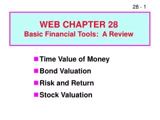
WEB CHAPTER 28 Basic Financial Tools: A Review. Time Value of Money Bond Valuation Risk and Return Stock Valuation. Time lines show timing of cash flows. 0. 1. 2. 3. i%. CF 0. CF 1. CF 2. CF 3.

E N D
WEB CHAPTER 28Basic Financial Tools: A Review • Time Value of Money • Bond Valuation • Risk and Return • Stock Valuation
Time lines show timing of cash flows. 0 1 2 3 i% CF0 CF1 CF2 CF3 Tick marksat ends of periods, so Time 0 is today; Time 1 is the end of Period 1; or the beginning of Period 2.
Time line for a $100 lump sum due at the end of Year 2. 0 1 2 Year i% 100
Time line for an ordinary annuity of $100 for 3 years. 0 1 2 3 i% 100 100 100
What’s the FV of an initial $100 after1, 2, and 3 years if i = 10%? 0 1 2 3 10% 100 FV = ? FV = ? FV = ? Finding FVs (moving to the right on a time line) is called compounding.
After 1 year: FV1 = PV + INT1 = PV + PV (i) = PV(1 + i) = $100(1.10) = $110.00. After 2 years: FV2 = PV(1 + i)2 = $100(1.10)2 = $121.00.
After 3 years: FV3 = PV(1 + i)3 = $100(1.10)3 = $133.10. In general, FVn = PV(1 + i)n.
What’s the FV in 3 years of $100 received in Year 2 at 10%? 0 1 2 3 10% 100 110
What’s the FV of a 3-year ordinary annuity of $100 at 10%? 0 1 2 3 10% 100 100 100 110 121 FV = 331
N I/YR PV PMT FV Financial Calculator Solution INPUTS 3 10 0 -100 331.00 OUTPUT Have payments but no lump sum PV, so enter 0 for present value.
What’s the PV of $100 due in 2 years if i = 10%? Finding PVs is discounting, and it’s the reverse of compounding. 0 1 2 10% 100 PV = ?
Solve FVn = PV(1 + i )n for PV: 2 1 PV = $100 = $100 PVIF i, n 1.10 = $100 0.8264 = $82.64.
What’s the PV of this ordinary annuity? 0 1 2 3 10% 100 100 100 90.91 82.64 75.13 248.69 = PV
N I/YR PV PMT FV INPUTS 3 10 100 0 OUTPUT -248.69 Have payments but no lump sum FV, so enter 0 for future value.
How much do you need to save each month for 30 years in order to retire on $145,000 a year for 20 years, i = 10%? months before retirement years after retirement 1 2 360 1 2 19 20 0 ... ... PMT PMT PMT -145k -145k -145k -145k
How much must you have in your account on the day you retire if i = 10%? years after retirement 0 1 2 19 20 ... ... -145k -145k -145k -145k How much do you need on this date?
N I/YR PV FV You need the present value of a20- year 145k annuity--or $1,234,467. INPUTS 20 10 -145000 0 PMT OUTPUT 1,234,467
How much do you need to save each month for 30 years in order to have the $1,234,467 in your account? You need $1,234,467 on this date. months before retirement 1 2 360 0 ... ... PMT PMT PMT
N I/YR PV FV You need a payment such that the future value of a 360-period annuity earning 10%/12 per period is $1,234,467. INPUTS 360 10/12 0 1234467 PMT OUTPUT 546.11 It will take an investment of $546.11 per month to fund your retirement.
Key Features of a Bond 1. Par value: Face amount; paid at maturity. Assume $1,000. 2. Coupon interest rate: Stated interest rate. Multiply by par value to get dollars of interest. Generally fixed. (More…)
3. Maturity: Years until bond must be repaid. Declines. 4. Issue date: Date when bond was issued.
PV annuity PV maturity value PV annuity $ 614.46 385.54 $1,000.00 = = = The bond consists of a 10-year, 10% annuity of $100/year plus a $1,000 lump sum at t = 10: INPUTS 10 10 100 1000 N I/YR PV PMT FV -1,000 OUTPUT
What would happen if expected inflation rose by 3%, causing r =13%? INPUTS 10 13 100 1000 N I/YR PV PMT FV -837.21 OUTPUT When rd rises, above the coupon rate, the bond’s value falls below par, so it sells at a discount.
What would happen if inflation fell, and rd declined to 7%? INPUTS 10 7 100 1000 N I/YR PV PMT FV -1,210.71 OUTPUT If coupon rate > rd, price rises above par, and bond sells at a premium.
The bond was issued 20 years ago and now has 10 years to maturity. What would happen to its value over time if the required rate of return remained at 10%, or at 13%,or at 7%?
Bond Value ($) rd = 7%. 1,372 1,211 rd = 10%. M 1,000 837 rd = 13%. 775 30 25 20 15 10 5 0 Years remaining to Maturity
At maturity, the value of any bond must equal its par value. • The value of a premium bond would decrease to $1,000. • The value of a discount bond would increase to $1,000. • A par bond stays at $1,000 if rd remains constant.
Economy Prob. T-Bill HT Coll USR MP Recession 0.10 8.0% -22.0% 28.0% 10.0% -13.0% Below avg. 0.20 8.0 -2.0 14.7 -10.0 1.0 Average 0.40 8.0 20.0 0.0 7.0 15.0 Above avg. 0.20 8.0 35.0 -10.0 45.0 29.0 Boom 0.10 8.0 50.0 -20.0 30.0 43.0 1.00 Assume the FollowingInvestment Alternatives
What is unique about the T-bill return? • The T-bill will return 8% regardless of the state of the economy. • Is the T-bill riskless? Explain.
Do the returns of HT and Collections move with or counter to the economy? • HT moves with the economy, so it is positively correlated with the economy. This is the typical situation. • Collections moves counter to the economy. Such negative correlation is unusual.
Calculate the expected rate of return on each alternative. ^ r = expected rate of return. ^ rHT = 0.10(-22%) + 0.20(-2%) + 0.40(20%) + 0.20(35%) + 0.10(50%) = 17.4%.
^ r HT 17.40% Market 15.00 USR 13.80 T-bill 8.00 Collections 1.74 • HT has the highest rate of return. • Does that make it best?
What is the standard deviationof returns for each alternative? = Standard deviation. .
. HT: = ((-22 - 17.4)2 0.10 + (-2 - 17.4)2 0.20 + (20 - 17.4)2 0.40 + (35 - 17.4)2 0.20 + (50 - 17.4)2 0.10)1/2 = 20.0%. T-bills = 0.0%. Coll = 13.4%. USR = 18.8%. M = 15.3%. HT = 20.0%.
The coefficient of variation (CV) is calculated as follows: ^ /r. CVHT = 20.0%/17.4% = 1.15 1.2. CVT-bills = 0.0%/8.0% = 0. CVColl = 13.4%/1.74% = 7.7. CVUSR = 18.8%/13.8% = 1.36 1.4. CVM = 15.3%/15.0% = 1.0.
Prob. T-bill USR HT 0 8 13.8 17.4 Rate of Return (%)
Standard deviation measures the stand-alone risk of an investment. • The larger the standard deviation, the higher the probability that returns will be far below the expected return. • Coefficient of variation is an alternative measure of stand-alone risk.
Expected Return versus Risk Expected Risk, CV Security return HT 17.4% 20.0% 1.2 Market 15.0 15.3 1.0 USR 13.8 18.8 1.4 T-bills 8.0 0.0 0.0 Collections 1.74 13.4 7.7 • Which alternative is best?
Portfolio Risk and Return Assume a two-stock portfolio with $50,000 in HT and $50,000 in Collections. ^ Calculate rp and p.
Portfolio Return, rp ^ ^ rp is a weighted average: n ^ ^ rp = wiri i = 1 ^ rp = 0.5(17.4%) + 0.5(1.74%) = 9.6%. ^ ^ ^ rp is between rHT and rColl.
Alternative Method Estimated Return Economy Prob. HT Coll. Port. Recession 0.10 -22.0% 28.0% 3.0% Below avg. 0.20 -2.0 14.7 6.4 Average 0.40 20.0 0.0 10.0 Above avg. 0.20 35.0 -10.0 12.5 Boom 0.10 50.0 -20.0 15.0 ^ rp = (3.0%)0.10 + (6.4%)0.20 + (10.0%)0.40 + (12.5%)0.20 + (15.0%)0.10 = 9.6%. (More...)
p = ((3.0 - 9.6)2 0.10 + (6.4 - 9.6)2 0.20 + (10.0 - 9.6)2 0.40 + (12.5 - 9.6)2 0.20 + (15.0 - 9.6)2 0.10)1/2 = 3.3%. • p is much lower than: • either stock (20% and 13.4%). • average of HT and Coll (16.7%). • The portfolio provides average return but much lower risk. The key here is negative correlation.
Portfolio standard deviation in general p= Portfolio standard deviation. Where w1 and w2 are portfolio weights and r1,2 is the correlation coefficient between stock 1 and 2.
Two-Stock Portfolios • Two stocks can be combined to form a riskless portfolio if r = -1.0. • Risk is not reduced at all if the two stocks have r = +1.0. • In general, stocks have r 0.65, so risk is lowered but not eliminated. • Investors typically hold many stocks. • What happens when r = 0?
Portfolio beta bp = Portfolio beta bp = w1b1 + w2b2 Where w1 and w2 are portfolio weights, and b1 and b2 are stock betas. For our portfolio of 50% HT and 50% Collections, bp = 0.5(1.30) + 0.5(-0.87) = 0.215 0.22.
What would happen to the riskiness of an average portfolio as more randomly picked stocks were added? • p would decrease because the added stocks would not be perfectly correlated, but rp would remain relatively constant. ^
Prob. Large 2 1 0 15 Return 135% ; Large20%.
p (%) Company-Specific (Diversifiable) Risk 35 Stand-Alone Risk, p 20 0 Market Risk 10 20 30 40 2,000+ # Stocks in Portfolio
Stand-alone Market Diversifiable = + . risk risk risk Market risk is that part of a security’s stand-alone risk that cannot be eliminated by diversification. Firm-specific, or diversifiable, risk is that part of a security’s stand-alone risk that can be eliminated by diversification.
Conclusions • As more stocks are added, each new stock has a smaller risk-reducing impact on the portfolio. • p falls very slowly after about 40 stocks are included. The lower limit for p is about 20% = M . • By forming well-diversified portfolios, investors can eliminate about half the riskiness of owning a single stock.