Chapter 9: The Analysis of Variance (ANOVA)
480 likes | 1.04k Vues
Chapter 9: The Analysis of Variance (ANOVA). http://www.luchsinger-mathematics.ch/Var_Reduction.jpg. ANOVA: Examples. Do four different brands of gasoline have different effects on automobile efficiency?

Chapter 9: The Analysis of Variance (ANOVA)
E N D
Presentation Transcript
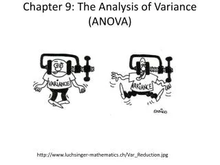
Chapter 9: The Analysis of Variance (ANOVA) http://www.luchsinger-mathematics.ch/Var_Reduction.jpg
ANOVA: Examples • Do four different brands of gasoline have different effects on automobile efficiency? • Does the type of sugar solution (glucose, sucrose, fructose, mixture) have an effect on bacterial growth? 3) Does the resulting color density of a fabric depend on the amount of dye used?
F Distribution http://www.vosesoftware.com/ModelRiskHelp/index.htm#Distributions/ Continuous_distributions/F_distribution.htm
P-value for an upper-tailed F test shaded area=P-value = 0.05
ANOVA Hypothesis test: Summary H0: μ1 = μ2 = = μk Ha: At least two μ’s are different Test statistic: P-value: area under the upper tail with an F distribution with (dfm, dfe) degrees of freedom
ANOVA: Example A random sample of 15 healthy young men are split randomly into 3 groups of 5. They receive 0, 20, and 40 mg of the drug Paxil for one week. Then their serotonin levels are measured to determine whether Paxil affects serotonin levels. The data is on the next slide. Does Paxil affect serotonin levels in healthy young men?
ANOVA: Example (cont) 1. Let 1 be the mean serotonin level for men receiving 0 mg of Paxil. Let 2 be the mean serotonin level for men receiving 20 mg of Paxil. Let 3 be the mean serotonin level for men receiving 40 mg of Paxil.
ANOVA: Example (cont) 2. H0: 1 = 2 = 3; mean serotonin levels are the same at all 3 dosage levels [or, mean serotonin levels are unaffected by Paxil dose] HA: The mean serotonin levels of the three groups are not all equal. [or, serotonin levels are affected by Paxil does]
Example: ANOVA (cont) 7. This does give strong support (0.001 < P < 0.01) to the claim that there is a difference in serotonin levels among the groups of men taking 0, 20, and 40 mg of Paxil. This does give strong support (0.001 < P < 0.01) to the claim that Paxil intake affects serotonin levels in young men.
Overall Risk of Type I Error in Using Repeated t Tests at = 0.05
Example: Tukey A biologist wished to study the effects of ethanol on sleep time. A sample of 20 rants matched for age and other characteristics, was selected, and each rat was given an oral injection having a particular concentration of ethanol per body weight. The rapid eye movement (REM) sleep time for each rat was then recorded for a 24-hour period with the results in the table on the next slide. Does the data indicate that the true average REM sleep time depends of the concentration of ethanol?
OUTPUT: Tukeycldiff The GLM Procedure Tukey'sStudentized Range (HSD) Test for sleep NOTE: This test controls the Type I experimentwise error rate. Alpha 0.05 Error Degrees of Freedom 16 Error Mean Square 92.9625 Critical Value of Studentized Range 4.04609 Minimum Significant Difference 17.446 Comparisons significant at the 0.05 level are indicated by ***. Difference amount Between Simultaneous 95% Comparison Means Confidence Limits 1 - 2 17.740 0.294 35.186 *** 1 - 3 31.360 13.914 48.806 *** 1 - 4 46.520 29.074 63.966 *** 2 - 1 -17.740 -35.186 -0.294 *** 2 - 3 13.620 -3.826 31.066 2 - 4 28.780 11.334 46.226 *** 3 - 1 -31.360 -48.806 -13.914 *** 3 - 2 -13.620 -31.066 3.826 3 - 4 15.160 -2.286 32.606 4 - 1 -46.520 -63.966 -29.074 *** 4 - 2 -28.780 -46.226 -11.334 *** 4 - 3 -15.160 -32.606 2.286
OUTPUT: Tukey lines The GLM Procedure Tukey'sStudentized Range (HSD) Test for sleep NOTE: This test controls the Type I experimentwise error rate, but it generally has a higher Type II error rate than REGWQ. Alpha 0.05 Error Degrees of Freedom 16 Error Mean Square 92.9625 Critical Value of Studentized Range 4.04609 Minimum Significant Difference 17.446 Means with the same letter are not significantly different. Tukey Grouping Mean N amount A 79.280 5 1 B 61.540 5 2 B C B 47.920 5 3 C C 32.760 5 4
Example: Dunnett A biologist wished to study the effects of ethanol on sleep time. A sample of 20 rants matched for age and other characteristics, was selected, and each rat was given an oral injection having a particular concentration of ethanol per body weight. The rapid eye movement (REM) sleep time for each rat was then recorded for a 24-hour period with the results in the table on the next slide. Does the data indicate that the true average REM sleep time is different for the ingestion of any alcohol?
OUTPUT: Dunnettcldiff The GLM Procedure Dunnett's t Tests for sleep NOTE: This test controls the Type I experimentwise error for comparisons of all treatments against a control. Alpha 0.05 Error Degrees of Freedom 16 Error Mean Square 92.9625 Critical Value of Dunnett's t 2.59232 Minimum Significant Difference 15.808 Comparisons significant at the 0.05 level are indicated by ***. Difference amount Between Simultaneous 95% Comparison Means Confidence Limits 2 - 1 -17.740 -33.548 -1.932 *** 3 - 1 -31.360 -47.168 -15.552 *** 4 - 1 -46.520 -62.328 -30.712 ***
Randomized Block Experiments Researchers are interested in the effect that acid has on growth rate of alfalfa plants. To control sunlight, the randomized block procedure is used.
Example: RBD An experiment was designed to study the performance of four different detergents in cleaning clothes. The clothes were measured on cleanness (higher= cleaner) after being stained with three different common stains and cleaned with the four detergents. We want to know which if any detergent is better.
Example: RBD (cont) 1. Let 1 be the mean cleaning value for detergent 1. Let 2 be the mean cleaning value for detergent 2. Let 3be the mean cleaning value for detergent 3. Let 4be the mean cleaning value for detergent .
Example: RBD (cont) 2. H0: 1= 2= 3= 4; mean cleaning levels for the 4 detergents are the same. HA: At least two of the detergents have different cleaning levels.
Example: RBD (cont) 7. This data does give strong support (P = 0.0063) to the claim that there is difference in how well the four detergents clean stains.
Example: RBD 2 An experiment was designed to study the performance of four different detergents in cleaning clothes. The clothes were measured on cleanness (higher= cleaner) after being stained with three different common stains and cleaned with the four detergents. We want to know if the stains (blocks) have an effect.
Example: RBD 2 (cont) 1. Let 1 be the mean cleaning value for stain 1. Let 2 be the mean cleaning value for stain 2. Let 3be the mean cleaning value for stain 3.
Example: RBD 2 (cont) 2. H0: 1= 2= 3= 4; mean cleaning levels for the 4 detergents are the same. HA: At least two of the detergents have different cleaning levels.
Example: RBD 2 (cont) 7. This data does give strong support (P = 0.0018) to the claim that there is difference in how well the detergents clean the different stains.
