Download
1 / 44
490 likes | 1.46k Vues
Operations Management Inventory Management Chapter 12 - Part I. Outline. Functions of Inventory. ABC Analysis. Inventory Costs . Inventory Models for Independent Demand. Economic Order Quantity (EOQ) Model. Production Order Quantity (POQ) Model. Quantity Discount Model.

E N D
Operations ManagementInventory ManagementChapter 12 - Part I
Outline • Functions of Inventory. • ABC Analysis. • Inventory Costs . • Inventory Models for Independent Demand. • Economic Order Quantity (EOQ) Model. • Production Order Quantity (POQ) Model. • Quantity Discount Model. • Probabilistic Models with Varying Demand. • Fixed Period Systems.
Types of Inventory • Raw materials. • Work-in-progress. • Maintenance/repair/operating (MRO) supply. • Finished goods.
The Functions of Inventory • To ”decouple” or separate various parts of the production process. • To smooth production (link supply and demand). • To provide goods for customers (quick response). • To take advantage of quantity discounts. • Buy more to get a reduced price. • To hedge against inflation and upward price changes (speculation). • Buy more now if you think price will rise.
Disadvantages of Inventory • High cost - $$$$$ • Money tied up in inventory could be better used elsewhere in the organization. • Difficult to control. • Inventories occur in many places. • Hides production problems. • Large inventories may overcome poor quality production or poor quality materials.
ABC Analysis • Divide inventory into 3 classes based on annual $ volume. • Annual $ volume = Annual demand x Unit cost. A class - Most important. 15-20% of products. 60-80% of value. B class -Less important. 20-40% of products. 15-30% of value. C class - Least important. 50-60% of products. 5-10% of value.
ABC Analysis • Sort products from largest to smallest annual $ volume. • Divide into A, B and C classes. • Focus on A products. • Develop class A suppliers more. • Give tighter physical control of A items. • Forecast A items more carefully. • Consider B products only after A products.
Classifying Items as ABC 25 products sorted by Annual $ Volume (Sales) Product Sales % 1 100 14 2 92 13 3 88 12 4 60 8 5 58 8 6 53 7 7 49 7 8 41 6 9 32 4 10 26 4 11 21 3 12 18 2 13 16 2 14-25 66 9 Total 720 100 80 Annual $ Usage (x1000) 60 40 20 0 20 10 15 1 25 5 Product
Classifying Items as ABC Class % $ Vol % Items A 39% 12% (3/25) 100 B 52% 40% (10/25) 80 C 9% 48% (12/25) Annual $ Usage (x1000) 60 A 40 20 B C 0 80 40 60 0 100 20 % of Products
Inventory Accuracy • Inventory accuracy importance: • To determine when and how much to order. • To achieve high level of service. • Information system tracks inventory, but… • Not all items sold are entered (scanned) properly. • Some items disappear without being sold (theft, defective, damaged, etc.)
Inventory Counting • Count products to verify inventory records. • Shut down facility and count everything at one time (once per year). • Cycle counting: count items continuously (count some each week). • Count A items most frequently (for example, once a month). • Count B items less frequently (twice a year). • Count C items least frequently (once a year).
Inventory for Services • Can be large $. • “Shrinkage” (theft) is a problem. • Often over 3%! • Good personnel selection, training, and discipline is key. • Establish tight control of shipments entering and leaving the facility. • Enforce procedures for documenting product movement. • Information systems can monitor inventory levels and help ensure accuracy.
Inventory Costs • Holding costs - Associated with holding or “carrying” inventory over time. • Ordering costs - Associated with costs of placing order and receiving goods. • Setup costs - Cost to prepare a machine or process for manufacturing an order. • Stockout costs- Cost of not making a sale and lost future sales.
Holding Costs • Investment costs (borrowing, interest). • Insurance. • Taxes. • Storage and handling. • Extra staffing. • Pilferage, damage, spoilage, scrap. • Obsolescence.
Category Investment costs Housing costs Material handling costs Labor cost from extra handling Pilferage, scrap, and obsolescence Cost as a % of Inventory Value 6 - 24% 3 - 10% 1 - 3.5% 3 -5% 2 - 5% Inventory Holding Costs – Usually 20-30% of Total
Ordering Costs To order and receive product: • Supplies. • Forms. • Order processing. • Clerical support. • etc.
Setup Costs To change equipment and setup for new product: • Clean-up costs. • Re-tooling costs. • Adjustment costs. • etc.
Stockout Costs For not making a sale and for lost future sales: - Customer may wait for a backorder, or - Cancel order (and acquire product elsewhere). • Backorder costs: expediting, special orders, rush shipments, etc. • Lost current sale cost. • Lost future sales (hard to estimate).
Inventory Questions • How much to order (each time)? • 100 units, 50 units, 23.624 units, etc. • When to order? • Every 3 days, every week, every month, etc. • When only 5 items are left, when only 10 items are left, when only 20 items are left, etc. • Many different models can be used, depending on nature of products and demand.
Independent vs. Dependent Demand • Independent demand - Demand for item is independent of demand for any other item. • Dependent demand - Demand for item depends upon the demand for some other item. • Example: Demand for car engines depends on demand for new cars. • We will consider only independent demand.
Inventory Models How much and when to order? • Fixed order-quantity models. • 1. Economic order quantity (EOQ). • 2. Production order quantity (POQ). • 3. Quantity discount. • Probabilistic models. • Fixed order-period models.
How Much and When to Order? • Given a fixed annual demand for a product. • With many small orders: • Amount on hand is always small, so inventory is small. • Frequent orders means cost of ordering is large. • With few large orders: • Amount on hand may be large (when order arrives), so inventory may be large. • Infrequent orders mean cost of ordering is small.
EOQ – Economic Order Quanitity Models • How much to order (each time)? • Order size is a constant = Q • Q is selected to minimize total cost. • When to order? • Order when amount remaining = ROP • ROP is selected so chance of running out is small.
EOQ Assumptions • Known and constant demand. • Known and constant lead time. • Instantaneous receipt of material. • No quantity discounts. • Only order cost and holding cost. • No stockouts.
EOQ Model - How Much to Order? Annual Cost Holding Cost Curve Order Cost Curve Order Quantity
EOQ Model - How Much to Order? Annual Cost Total Cost Curve Holding Cost Curve Order Cost Curve Order Quantity Optimal Order Quantity (EOQ=Q*)
Why Holding Costs Increase • For fixed annual demand, larger order quantities means: • Larger inventory (larger amount ordered each time). • Larger inventory holding cost. • Example: Annual demand = 1200 units • Order 600 each time. • Maximum inventory = 600 • Order 50 each time. • Maximum inventory = 50
Why Order Costs Decrease • For fixed annual demand, larger order quantities means: • Fewer orders per year. • Smaller order cost per year. • Example: Annual demand = 1200 units • Order 600 each time. • 1200/600 = 2 orders per year. • Order 50 each time. • 1200/50 = 24 orders per year.
Deriving an EOQ • Develop an expression for total costs. • Total cost = order cost + holding cost • Find order quantity that gives minimum total cost (use calculus). • Minimum is when slope is flat. • Slope = Derivative. • Set derivative of total cost equal to 0 and solve for best order quantity.
D = = Expected Number of Orders per year N Q D S Order Cost per year = Q (average inventory level) H = Holding Cost per year EOQ Model Equations D = Annual demand (relatively constant) S = Order cost per order H = Holding (carrying) cost per unit per year d = Demand rate (units per day, units per week, etc.) L = Lead time (constant) (in days, weeks, hours, etc.) Determine: Q = Order size (number of items per order) Given
Inventory Level Order Quantity(Q) AverageInventory (Q/2) 0 Time EOQ Model - Average Inventory Level Maximum inventory = Q Minimum inventory = 0
D = = Expected Number of Orders per year N Q D S Order Cost per year = Q (average inventory level) H = = Holding Cost per year EOQ Model Equations D = Annual demand (relatively constant) S = Order cost per order H = Holding (carrying) cost per unit per year d = Demand rate (units per day, units per week, etc.) L = Lead time (constant) (in days, weeks, hours, etc.) Determine: Q = Order size (number of items per order) Given Q H 2
EOQ Model - How Much to Order? Annual Cost Total Cost Curve = (D/Q)S+(Q/2)H Holding Cost =(Q/2)H Order Cost Curve = (D/Q)S Order Quantity Optimal Order Quantity (EOQ=Q*)
D 1 S + H = 0 Q2 2 D Q = Total Cost S + H Q 2 EOQ Total Cost Optimization Take derivative of total cost with respect to Q and set equal to zero: Solve for Q to get optimal order size: × × 2 D S EOQ = Q* = H
D = = Expected Number of Orders N Q* Working Days / Year Expected Time Between Orders = = T N EOQ Model Equations D = Annual demand S = Order cost per order H = Holding (carrying) cost × × 2 D S Optimal Order Quantity = = Q* H
EOQ Model - When to order? D = Annual demand (relatively constant) d = Demand per day L = Lead time in days Determine: ROP = reorder point (number of pieces or items remaining when order is to be placed) Given D Suppose demand is 10 per day and lead time is (always) 4 days. When should you order? When 40 are left! = d Working Days / Year = × ROP d L
Lead Time = time between placing and receiving an order Reorder Point (ROP) 4th order 2nd order 3rd order 1st order received 1st order placed EOQ Model - When To Order Inventory Level Q* Time
EOQ Example Demand = 1200/year Order cost = $50/order Holding cost = $5 per year per item 260 working days per year 2 ×1200 ×50 = = 154.92 units/order; so order 155 each time Q* 5 1200/year Expected Number of Orders = N = = 7.74/year 155 260 days/year Expected Time Between Orders = T = = 33.6 days 7.74/year 1200 155 Total Cost = 50 + 5 = 387.10 + 387.50 = $774.60/year 155 2
1200 Q Total Cost = 50 + 5 Q 2 EOQ is Robust Demand = 1200/year Order cost = $50/order Holding cost = $5 per year per item 260 working days per year Q = 155 units/order TC = $774.60/year Q* = 154.92 units/order TC = $774.60/year = 387.30 + 387.30 Suppose we must order in multiples of 20: Q = 140 units/order TC = $778.57/year (+0.5%) Q = 160 units/order TC = $775.00/year (+0.05%) Cost is nearly optimal!
1200 Q Total Cost = 50 + 5 Q 2 EOQ is Robust Demand = 1200/year Order cost = $50/order Holding cost = $5 per year per item 260 working days per year Q = 155 units/order TC = $774.60/year Q* = 154.92 units/order TC = $774.60/year = 387.30 + 387.30 Suppose we wish to order 6 times per year (every 2 months): Q = 1200/6 = 200 units/order(200/order is 29% above Q*) TC = $800.00/year = 300.00 + 500.00 (Cost is only 3.3% above optimal: $800 vs. $774.60)
EOQ Model is Robust Annual Cost Total Cost Curve Small variation in cost Order Quantity 154.92 Large variation in order size
Robustness • EOQ amount can be adjusted to facilitate business practices. • If order size is reasonably near optimal (+ or - 20%), then cost will be very near optimal (within a few percent). • If parameters (order cost, holding cost, demand) are not known with certainty, then EOQ is still very useful.
EOQ Model - When to order? Demand = 1200/year Order cost = $50/order Holding cost = $5 per year per item 260 working days per year Lead time = 5 days 1200/year = = 4.615/day d 260 days/year ROP = 4.615 units/day 5 days = 23.07 units -> Place an order whenever inventory falls to (or below) 23 units