Basic Concepts of Relational Databases
610 likes | 742 Vues
This article provides an overview of relational databases, focusing on key concepts such as tables, records, and operations in relational algebra. We explore how records in a table are conceptually unordered, the significance of attributes, and whether duplicate records are allowed. The piece delves into basic operations like selection, projection, set-difference, union, and cross-product, explaining their functionalities and results. Additionally, it discusses the SQL syntax for querying data, introduces aggregate functions, and highlights efficient query evaluation strategies.

Basic Concepts of Relational Databases
E N D
Presentation Transcript
Example Instances R1 • A table or relation stores records (or tuples) that have the same attributes • Order of records is not important conceptually • “Sailors” and “Reserves” relations for our examples. • Questions: Can we have two records with the same sid in the same sailor (e.g., S1 or S2) table? • Can the same sailor reserve the same boat many times? S1 S2
Relational Algebra • Basic operations: • Selection (cR ) Selects the subset of rows that satisfy a condition c from R. • Projection (listR ) Keeps only the attributes in list from R. • Set-difference ( R1–R2) Finds tuples in R1, but not in R2. • Union(R1R2) Finds tuples that belong to R1 or R2. • Cross-product(R1xR2) Allows us to combine two relations. • Renaming(p RnewRold)Allows us to rename a relation Rold to Rnew. • Additional operations: • Intersection, join, division: Not essential, but (very!) useful. • Since each operation returns a relation, operationscan be composed! (Algebra is “closed”.)
Projection • Deletes attributes that are not in projection list. • Schema of result contains exactly the fields in the projection list, with the same names that they had in the (only) input relation. • The formal projection operator has to eliminate duplicates! • Note: real systems typically don’t do duplicate elimination unless the user explicitly asks for it.
Selection • Selects rows that satisfy selection condition. • No duplicates in result! (Why?) • Schema of result identical to schema of (only) input relation. • Result relation can be the input for another relational algebra operation! (Operatorcomposition.)
Union, Intersection, Set-Difference • All of these operations take two input relations, which must be union-compatible: • Same number of fields. • Corresponding fields have the same type.
Cross (Cartesian)-Product, X • Each row of S is paired with each row of R. • Result schema has one field per field of S and R, with field names `inherited’ if possible. • Conflict: Both S and R have a field called sid.
Joins • Condition Join: • Result schema same as that of cross-product. • Fewer tuples than cross-product, might be able to compute more efficiently • Sometimes called a theta-join.
Joins • Equi-Join: A special case of condition join where the condition c contains only equalities. • Result schema similar to cross-product, but only one copy of fields for which equality is specified. • Natural Join: Equijoin on all common fields.
Basic SQL Query SELECT [DISTINCT] target-list FROMrelation-list WHERE qualification • target-list A list of attributes of relations in relation-list • relation-list A list of relation names (possibly with a range-variable after each name). • qualification Comparisons (Attr op const or Attr1 op Attr2, where op is one of <,>.=,,,) combined using AND, OR and NOT. • DISTINCT is an optional keyword indicating that the answer should not contain duplicates. Default is that duplicates are not eliminated!
Conceptual Evaluation Strategy • Semantics of an SQL query defined in terms of the following conceptual evaluation strategy: • Compute the cross-product of relation-list. • Discard resulting tuples if they fail qualifications. • Delete attributes that are not in target-list. • If DISTINCT is specified, eliminate duplicate rows. • This strategy is probably the least efficient way to compute a query! An optimizer will find more efficient strategies to compute the same answers.
Example of Conceptual Evaluation SELECT S.sname FROM Sailors S, Reserves R WHERE S.sid=R.sid AND R.bid=103
A Note on Range Variables • Really needed only if the same relation appears twice in the FROM clause. The previous query can also be written as: SELECT S.sname FROM Sailors S, Reserves R WHERES.sid=R.sid AND bid=103 OR SELECT sname FROM Sailors, Reserves WHERE Sailors.sid=Reserves.sid AND bid=103
Find sid’s of sailors who’ve reserved a red or a green boat Set Operations - Union • UNION: Can be used to compute the union of any two union-compatible sets of tuples (which are themselves the result of SQL queries). • If we replace ORby ANDin the first version, what do we get? • Do we need the Sailors table? • Also available: EXCEPT (corresponds to the set difference operation of relational algebra) • What do we get if we replace UNIONby EXCEPT? SELECT S.sid FROM Sailors S, Boats B, Reserves R WHERE S.sid=R.sid AND R.bid=B.bid AND (B.color=‘red’ OR B.color=‘green’) SELECT S.sid FROM Sailors S, Boats B, Reserves R WHERE S.sid=R.sid AND R.bid=B.bid AND B.color=‘red’ UNION SELECT S.sid FROM Sailors S, Boats B, Reserves R WHERE S.sid=R.sid AND R.bid=B.bid AND B.color=‘green’
COUNT (*) COUNT ( [DISTINCT] A) SUM ( [DISTINCT] A) AVG ( [DISTINCT] A) MAX (A) MIN (A) Aggregate Operators • Significant extension of relational algebra. single column SELECT COUNT (*) FROM Sailors S SELECT S.sname FROM Sailors S WHERE S.rating= (SELECT MAX(S2.rating) FROM Sailors S2) SELECT AVG (S.age) FROM Sailors S WHERE S.rating=10 SELECT COUNT (DISTINCT S.rating) FROM Sailors S WHERE S.sname=‘Bob’ SELECT AVG ( DISTINCT S.age) FROM Sailors S WHERE S.rating=10
GROUP BY and HAVING • So far, we’ve applied aggregate operators to all (qualifying) tuples. Sometimes, we want to apply them to each of several groups of tuples. • Consider: Find the age of the youngest sailor for each rating level. • In general, we don’t know how many rating levels exist, and what the rating values for these levels are! • Suppose we know that rating values go from 1 to 10; we can write 10 queries that look like this (!): SELECT MIN (S.age) FROM Sailors S WHERE S.rating = i For i = 1, 2, ... , 10:
Queries With GROUP BY and HAVING • The target-list contains (i) an attribute list(ii) terms with aggregate operations (e.g., MIN (S.age)). • Theattribute list (i)must be a subset of grouping-list. Intuitively, each answer tuple corresponds to a group, andthese attributes must have a single value per group. (A group is a set of tuples that have the same value for all attributes in grouping-list.) SELECT [DISTINCT] target-list FROMrelation-list WHERE qualification GROUP BYgrouping-list HAVING group-qualification
For each red boat, find the number of reservations for this boat • Grouping over a join of two relations. • We cannot remove B.color=‘red’ from the WHERE clause and add a HAVING clause with this condition. Only columns that appear in the Group-By can appear in HAVING, unless they are arguments of an aggregate operator in HAVING. SELECT B.bid, COUNT (*) AS scount FROM Boats B, Reserves R WHERE R.bid=B.bid AND B.color=‘red’ GROUP BY B.bid
Basic Concepts of Indexing • Indexing mechanisms used to speed up access to desired data. • E.g., author catalog in library • Search Key - attribute to set of attributes used to look up records in a file. • An index fileconsists of records (called index entries) of the form • Index files are typically much smaller than the original file • Two basic kinds of indices: • Ordered indices: search keys are stored in sorted order • Hash indices: search keys are distributed uniformly across “buckets” using a “hash function”. pointer search-key
Ordered Indices • In an ordered index, index entries are stored sorted on the search key value. E.g., author catalog in library. • Primary index: in a sequentially ordered file, the index whose search key specifies the sequential order of the file. • Also called clustering index • The search key of a primary index is usually but not necessarily the primary key • Secondary index:an index whose search key specifies an order different from the sequential order of the file. Also called non-clustering index. • Index-sequential file: ordered sequential file with a primary index (also called ISAM - indexed sequential access method).
Dense Index Files • Dense index — Index record appears for every search-key value in the file (in this example we have clustering index).
Sparse Index Files • Sparse Index: contains index records for only some search-key values. • Applicable when records are sequentially ordered on search-key (i.e., only applicable to clustering indexes) • To locate a record with search-key value K we: • Find index record with largest search-key value <= K • Search file sequentially starting at the record to which the index record points • Less space and less maintenance overhead for insertions and deletions. • Generally slower than dense index for locating records. • Good tradeoff: sparse index with an index entry for every block in file, corresponding to least search-key value in the block.
Multilevel Index • If primary index does not fit in memory, access becomes expensive. • To reduce number of disk accesses to index records, treat primary index kept on disk as a sequential file and construct a sparse index on it. • outer index – a sparse index of primary index • inner index – the primary index file • If even outer index is too large to fit in main memory, yet another level of index can be created, and so on. • Indices at all levels must be updated on insertion or deletion from the file.
B+-Tree Index • All paths from root to leaf are of the same length (i.e., balanced tree) • Each node has between n/2 and n pointers. Each leaf node stores between (n–1)/2 and n–1 values. • n is called fanout (it corresponds to the maximum number of pointers/children). The value (n-1)/2 is called order (it corresponds to the minimum number of values). • Special cases: • If the root is not a leaf, it has at least 2 children. • If the root is a leaf (that is, there are no other nodes in the tree), it can have between 0 and (n–1) values. A B+-tree is a rooted tree satisfying the following properties:
Example of non-clustering (secondary) B+-tree on candidate key
Inserting a Data Entry into a B+ Tree • Find correct leaf L. • Put data entry onto L. • If L has enough space, done! • Else, must splitL (into L and a new node L2) • Redistribute entries evenly, copy upmiddle key. • Insert index entry pointing to L2 into parent of L. • This can happen recursively • To split index node, redistribute entries evenly, but push upmiddle key. (Contrast with leaf splits.) • Splits “grow” tree; root split increases height. • Tree growth: gets wider or one level taller at top.
Deleting a Data Entry from a B+ Tree • Start at root, find leaf L where entry belongs. • Remove the entry. • If L is at least half-full, done! • If L less that half-full, • Try to re-distribute, borrowing from sibling (adjacent node to the right). • If re-distribution fails, mergeL and sibling. • If merge occurred, must delete entry (pointing to L or sibling) from parent of L. • Merge could propagate to root, decreasing height.
B+-tree Update Examples • Consider the B+-tree below with order 2 (each node except for the root must contain at least two search key values – and 3 pointers). Show the tree that would result after successively applying each of the following operations. Remove 1 Remove 41
B+-tree Update Examples (cont) After removing 41 Remove 3 Insert 41
B+-tree Update Examples (cont) After inserting 41 Insert 1
3* 6* 9* 10* 11* 12* 13* 23* 31* 36* 38* 41* 44* 4* 20* 22* 35* Bulk Loading of a B+ Tree • If we have a large collection of records, and we want to create a B+ tree on some field, doing so by repeatedly inserting records is very slow. • Bulk Loadingcan be done much more efficiently. • Initialization: Sort all data entries (using external sorting), insert pointer to first (leaf) page in a new (root) page. Root Sorted pages of data entries; not yet in B+ tree
Bulk Loading (Cont.) • Index entries for leaf pages always entered into right-most index page just above leaf level. When this fills up, it splits. (Split may go up right-most path to the root.) • Much faster than repeated inserts! Root 10 20 Data entry pages 6 12 23 35 not yet in B+ tree 3* 6* 9* 10* 11* 12* 13* 23* 31* 36* 38* 41* 44* 4* 20* 22* 35* Root 20 10 Data entry pages 35 not yet in B+ tree 6 23 12 38 3* 6* 9* 10* 11* 12* 13* 23* 31* 36* 38* 41* 44* 4* 20* 22* 35*
Hash Indices • Hashing can be used not only for file organization, but also for index-structure creation. • A hash index organizes the search keys, with their associated record pointers, into a hash file structure. • Strictly speaking, hash indices are always secondary indices • if the file itself is organized using hashing, a separate primary hash index on it using the same search-key is unnecessary.
Hash Functions • In the worst case, the hash function maps all search-key values to the same bucket; this makes access time proportional to the number of search-key values in the file. • Ideal hash function is random, so each bucket will have the same number of records assigned to it irrespective of the actual distribution of search-key values in the file. • Typical hash functions perform computation on the internal binary representation of the search-key. • For example, for a string search-key, the binary representations of all the characters in the string could be added and the sum modulo the number of buckets could be returned.
External Sorting (disk-resident files) • Merging Sorted Files with 3 pages of main memory buffer sorted file 2 sorted file 1 merged file …
External Sorting (disk-resident files) sorted file 2 sorted file 1 merged file (1,…) (2,…) (4,…) write page to disk (5,…) bring next page of file 2 bring next page of file 1 (6,…) (7,…) (9,…) write page to disk (10,…) (11,…)
External Sorting (disk-resident files) Continuing the previous example: Question: I assumed that each file is already sorted. If the file is not sorted, how do I sort it (using only my 3 buffer pages?) Answer: Each file in the example is only 2 pages. Therefore, I can bring the entire file in memory, and sort it using any main-memory algorithm. Question: The previous example assumes two separate files. How do I apply this idea to sort a single file? Answer: You can split the file in two parts and merge them as if they were separate files. Question: Can I do better if I have M>3 main memory pages. Answer: Yes, instead of 2 you can merge up to M-1 files (because you need 1 page for writing the output).
Sorting a file that has 108 pages, using only 5 pages of main memory.
Basic Steps in Query Processing • Parsing and translation • translate the query into its internal form. This is then translated into relational algebra. • Parser checks syntax, verifies relations • Evaluation • The query-execution engine takes a query-evaluation plan, executes that plan, and returns the answers to the query.
Basic Steps in Query Processing : Optimization • A relational algebra expression may have many equivalent expressions • E.g., balance2500(balance(account)) is equivalent to balance(balance2500(account)) • Each relational algebra operation can be evaluated using one of several different algorithms • Correspondingly, a relational-algebra expression can be evaluated in many ways. • Annotated expression specifying detailed evaluation strategy is called an evaluation-plan. • E.g., can use an index on balance to find accounts with balance < 2500, • or can perform complete relation scan and discard accounts with balance 2500
Selection Operation • File scan – search algorithms that locate and retrieve records that fulfill a selection condition. • Algorithm A1 (linear search). Scan each file block and test all records to see whether they satisfy the selection condition. • Cost estimate (number of disk blocks scanned) = br • br denotes number of blocks containing records from relation r • If selection is on a key attribute, cost = (br /2) • stop on finding record • Linear search can be applied regardless of • selection condition or • ordering of records in the file, or • availability of indices
Selection Operation (Cont.) • A2 (binary search). Applicable if selection is an equality comparison on the attribute on which file is ordered. • Assume that the blocks of a relation are stored contiguously • Cost estimate (number of disk blocks to be scanned): • log2(br) — cost of locating the first tuple by a binary search on the blocks • Plus number of blocks containing records that satisfy selection condition
Selections Using Indices • Index scan – search algorithms that use an index • selection condition must be on search-key of index. • A3 (primary index on candidate key, equality). Retrieve a single record that satisfies the corresponding equality condition • Cost = HTi+ 1 (HTi is the height of the tree index) • A4 (primary index on nonkey, equality) Retrieve multiple records. • Records will be on consecutive blocks • Cost = HTi+ number of blocks containing retrieved records • A5 (equality on search-key of secondary index). • Retrieve a single record if the search-key is a candidate key • Cost = HTi+ 1 (if hash index HTi = 1 or HTi = 1.2 if we assume that there exist overflow buckets) • Retrieve multiple records if search-key is not a candidate key • Cost = HTi+ number of records retrieved • Can be very expensive! • each record may be on a different block • one block access for each retrieved record
Selections Involving Comparisons • Can implement selections of the form AV (r) or A V(r) by using • a linear file scan or binary search, • or by using indices in the following ways: • A6 (primary index, comparison). (Relation is sorted on A) • For A V(r) use index to find first tuple v and scan relation sequentially from there • For AV (r) just scan relation sequentially till first tuple > v; do not use index • A7 (secondary index, comparison). • For A V(r) use index to find first index entry v and scan index sequentially from there, to find pointers to records. • For AV (r) just scan leaf pages of index finding pointers to records, till first entry > v • In either case, retrieve records that are pointed to • requires an I/O for each record • Linear file scan may be cheaper if many records are to be fetched!