Download
1 / 40
420 likes | 652 Vues
New Experimental Test of Coulomb’s Law: A Laboratory Upper Limit on the Photon Rest Mass. A lecture on the Article. E.R. Williams, J. E. Faller and H.A. Hill (1971). Porat Amit & Oren Zarchin. Abstract. A high-frequency test of Coulomb’s law is described.

E N D
New Experimental Test of Coulomb’s Law:A Laboratory Upper Limit on the Photon Rest Mass A lecture on the Article E.R. Williams, J. E. Faller and H.A. Hill (1971) Porat Amit & Oren Zarchin
Abstract A high-frequency test of Coulomb’s law is described. The sensitivity of the experiment is given in terms of a finite photon rest mass, using the Proca equations. The null result of our measurement expressed in the form of the photon rest mass squared is
Abstract • Expressed as a deviation from Coulomb’s law of the form , our experiment gives . This result extends the validity of Coulomb’s law by two orders of magnitude.
Coulomb,Charles(1736-1806) • French physicist who performed experiments with a torsion balance. • His investigations led him to suggest that there were two "fluids" of electricity and magnetism. • He showed both forces were inverse square, and stated that they were unconnected separate phenomena. • The inverse square of electricity has come to be known as Coulomb's law.
Historical review • Using a Torsion balance Coulomb demonstrated directly that two like charges repel each other with a force varies inversely as the square distance between them.
Robinson,John(ca.1725-?) • English doctor who, in 1769, measured electrical repulsion went as r-2.06 and attraction as r-c where c < 2. From these results he surmised r-2 was correct. This determination was made before Coulomb proposed just this result, now know as Coulomb's law.
A deviation from Coulomb’s law? • A photon with a finite rest mass will cause a deviation, according to Proca equations. • A deviation from the Euclidian space can cause a deviation from the r square law. • This effect will be neglected when calculating a deviation due to the existence of a photon rest mass which varies from zero.
Historical review • Cavendish (1773) noted that if the force between charges obeys the inverse square law there should be no electric forces (I.e. electric fields) inside a hollow charge free cavity inside a conductor. • Maxwell has found that the exponent of r in Coulomb’s law could differ from two by less than 1/21600.
Historical review • Plimpton and Lawton (1936) charged an outer sphere with a lowly varying alternating current and detected the potential difference between the inner and outer spheres. They reduced Maxwell’s limit to 2x10⁻⁹. • Bartlett Goldhagen & Phillips (1970) achieved an upper limit of 1.3x10⁻¹³ .
Bartlett Goldhagen & Phillips (1970) • Using five concentric spheres, and applying a potential difference of 40 KV at 2500Hz between the outer spheres. • The potential difference between the inner two spheres was read using a Lock-in detector.
Theory- Proca equations • In conventional electrodynamics the mass of the photon is assumed to vanish. However, a finite photon mass may be accommodated in a unique way by changing the inhomogeneous Maxwell equations to the Proca equations. • Let us explain the basic concepts which lead to these equations
Some topics in Quantum Electrodynamics • The description of the interaction between the electromagnetic field and the electron-positron field constitutes the main problem of QED. • We will look on a combination of Maxwell equations with the Dirac form of the current (comes from the solution of Dirac equation). • The high-energy experiments test QED in a situation where the four-momentum transfer characteristic of the experiment, is as large as possible. The verdict, as far as the high-energy tests are concerned, is that the Maxwell equations with the Dirac form of the current for the electron and Muon are correct.
The electromagnetic field • We can describe the electromagnetic field by means of the equation of retarded potentials A=j (=1,2,3,4) • A is the potential of the electric field. • j is the current describing the charged particles • is the solution for Dirac equation for a particle interacting with an electromagnetic field. • is related to the Dirac operators.
Adding the photon’s mass • If the photon has a mass m0, an additional term is required A+ 2A = j • Where (should be h bar). • The equation show explicitly that the additional current term is proportional to the four vector potential A. Therefore they have a mutual influence.
Finally- Proca equation • Proca equation for a particle of spin 1 and mass m0 (such a photon) is A+ 2A = (4/c)j. • In a three dimensional notation, Gauss’s law becomes (1)
Developing the necessary equations • In order to calculate the sensitivity of the system, consider an idealized geometry consisting of two concentric, conducting, spherical shells of radii R2 > R1 with an inductor parallel with this spherical capacitor. • To the outer shell is applied a potential V0eiwt.
Developing the necessary equations • forming a spherical Gaussian surface at radius r between the two shells and then using the approximation for this interior region, the integral of Equation(1) over the volume interior to the Gaussian surface becomes (2)
Developing the necessary equations • Therefore E(r) is given by • (3) • Where q is the total charge on the inner shell. • A complete solution of the fields inside a symmetrically charged single sphere will give, after neglecting second order terms in the electrical filed , equation (3) and H=0.
Approaching the final equation • Since inside, • The voltage appearing across the inductor is then simply given by (4)
Approaching the final equation • The differential equation, which describes a regular LCR equation is • In the case of a nonzero rest mass
notes • Analyzing the signal to noise ratio of the system (conventional circuit theory) results that the use of • High frequency • High Q circuits • Large apparatus • High V0 Will serve to maximize the experimental sensitivity.
Experimental Setup • Charging a conducting shell (1.5m in diameter-Large) with 10KVolts peak to peak with a 4Mhz Sinusoidal voltage. Is it all?
Fiber optics • We would like to transmit data, to and from the inner sphere. • We cannot use Electrical wires since they will efffect the measurment. • So we use Fiber Optics, through a hole in the sphere. • In order to prevent penatration of Outer fields through the hole, we use the fiber as a Waveguide. • The waveguide diameter must be smaller than the cutoff frequency.
Noise • stray electric and magnetic fields
Noise - Solution • Adding 3 shells in order to prevent stray electric and magnetic fields inside the sphere. There is another problem..
Another Noise • Johnson effect = • gives noise of
Adding a Lockin Amplifier Phase shift Lockin Amplifier
Lock in amplifier Phase shift x Low pass filter filter
Lock in Amplifier Push pull signals signal RC vout • when the reference signal is positive, the signal goes out with no changes. • when the reference signal is negative, the signal goes out up side down. • The RC integrates over the signal and cancels same areas with negative sine. reference relay
Lock In Amplifier Demonstration • when the reference signal is positive, the signal goes out with no changes. • when the reference signal is negative, the signal goes out up side down. • The RC integrates over the signal and cancels same areas with negative sine.
A full view of the system • We need to check the System!
Calibration capacitor Light beam Checking & calibration • During a data run, to ensure that our system works properly. • A calibration Voltage is periodically introduced into the system on a third light beam while the reference beam is working. • On striking a light sensitive diode induces a voltage on the capacitor.
Calibration results • The calibration was done Over 3 cycles .
Notes • As high as possible applied voltage , serves to maximize the experimental accuracy . • In the experiment we use high frequencies in order to reduce the skin depth which varies as
Results • The experimental result is statistically consistent with the assumption that the photon rest mass is identically zero.
references • E. R. Williams, J. E. Faller, H. A. Hill. Phys. Rev. Let. 26 721 (1971) • Metrology and Fundamental Constants (oxford 1980) • D. F. Bartlett, P. E. Goldhagen, E. H. Phillips. Phys. Rev. D2 483 (1970) • Alfred S. Goldhaber, Michael Martin Nieto. Phys. Rev. Lett. 21 567 (1968) • S.J. Plimpton, W. E. Lawton. Phys. Rev. 50 1066 (1936) • יישומים של אפנון קרני לייזר • Varying Internet sites