An Introduction to Helioseismology (Global)
450 likes | 778 Vues
An Introduction to Helioseismology (Global). 2008 Solar Physics Summer School June 16-20, Sacramento Peak Observatory, Sunspot, NM. Special Acknowledgments. Rachel Howe Rudi Komm Frank Hill ( National Solar Observatory ) . Global Helioseismology. What is helioseismology?

An Introduction to Helioseismology (Global)
E N D
Presentation Transcript
An Introduction to Helioseismology(Global) 2008 Solar Physics Summer School June 16-20, Sacramento Peak Observatory, Sunspot, NM
Special Acknowledgments Rachel Howe Rudi Komm Frank Hill ( National Solar Observatory )
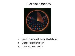
Global Helioseismology What is helioseismology? A bit of early history Basics p-modes and g-modes Spherical harmonics Observations Instrumentation Networks and spacecraft Time series Spectra Methods Peak finding Inversions Results Internal Properties of the Sun Solar Cycle variations
The early “days” of helioseismology • Discovered in 1960 that the solar surface is rising and falling with a 5-minute period • Many theories of wave physics postulated: • Gravity waves or acoustic waves or MHD waves? • Where was the region of propagation? • A puzzle – every attempt to measure the characteristic wavelength on the surface gave a different answer
The k- (diagnostic) diagram • Acoustic waves trapped within the internal temperature gradient predicted a specific dispersion relation between frequency and wavelength • A wide range of wavelengths are possible, so every early measurement was correct – result depended on aperture size • Observationally confirmed in 1975 • Max amplitude 20 cm/s
What is helioseismology? Helioseismology utilizes waves that propagate throughout the Sun to measure its invisible internal (and external) structure and dynamics.
Three types of modes • G(ravity) Modes – restoring force is buoyancy – internal gravity waves • P(ressure) Modes – restoring force is pressure • F(undamental) Modes – restoring force is buoyancy modified by density interface – surface gravity waves
Wave trapping • G modes exist where ω < N2 (Brunt-Väisälä frequency) • P modes exist where ω < ωac (acoustic cut-off frequency) and ω > S (Lamb frequency) • F modes are analogous to surface water waves
The P modes • A p mode is a standing acoustic wave. • Each mode can be described by a spherical harmonic. • Quantum numbers n (radial order), l (degree), and m (azimuthal order) identify the mode.
Spherical Harmonics l=6 m=0 l=6 m=3 l=6 m=6 • The harmonic degree, l, indicates the number of node lines on the surface, which is the total number of planes slicing through the Sun. • The azimuthal number m, describes the number of planes slicing through the Sun longitudinally. • - l ≤ m ≤ l • Picture credits: Noyes, Robert, "The Sun", in _The New Solar System_, J. Kelly Beatty and A. Chaikin ed., Sky Publishing Corporation, 1990, pg. 23.
Temporal Frequency units • ν = 1/(Period in seconds), units are Hertz (Hz) • ω = 2π/(Period in seconds), units are radians/sec • P = 5 min = 300 sec, ν = 3.33 mHz or 3333.33 μHz; ω = 2.1 ´ 10-2 rad/s Spatial Frequency units • kh = √(l(l+1)/Rsun (Mm-1)
Ray Paths Turning points
Duvall law • Modes turn at depth where sound speed = horizontal phase speed = ν/ℓ • So, all modes with same ν/ℓ must take same time to make one trip between reflections
Rotational Splitting • In absence of rotation, have standing wave pattern and degenerate case – the frequency 0 ( = /2) is independent of m • In presence of rotation, prograde and retrograde waves have different • Observed frequency n,l,m = 0 + δ where δ is the splitting frequency • IF the Sun rotated uniformly --> δ depend linearly on m.
An Observational Problem • The sun sets at a single terrestrial site, producing periodic time series gaps • The solar acoustic spectrum is convolved with the temporal window spectrum, contaminating solar spectrum with many spurious peaks
Solutions • Antarctica – max 6 month duration • Network – BiSON, IRIS, GONG – needs data merging, but maintainable • Space – SoHO: MDI, GOLF,VIRGO
Networks • 6-site network of single-pixel instruments, data since 1976, completed 1992. • Modes up to l=4 • Run by University of Birmingham, UK
Networks • Six stations around the world for continual coverage. • 256x256 pixels 1995-2001 • 1024 pixels since 2001 • Run from NSO Tucson.
Space Instruments 1996 - Present Coming Soon…. MDI GOLF VIRGO HMI
X = X = X = Observing Time Series Σ
Observing & processing challenges • Image geometry is paramount • Image scale affects ℓ-scale • Angular orientation mixes m-states • Fitting of spectral features not trivial • Can only view portion of solar surface, so have spatial leakage
Solar Acoustic Spectra - Diagram -m- Diagram m- Diagram
Fitting the Spectrum Standard model is a Lorentzian profile
Fitting the Spectrum Considerations: • Observations in Velocity and Intensity • Asymmetric Profile • Leakage matrix
Modes of different m cover different latitude ranges, giving latitudinal resolution. Inversions • Modes are reflected due to density variations. • The lower the l, the fewer surface reflections, and the deeper the mode penetrates. • Combining information from different modes lets us build up a picture of properties at different depths.
The (rotation) inversion problem Kernel Coefficients to be found Averaging Kernel
Eigenfunctions & Kernels • Inversion kernels constructed from eigenfunctions weighted by density
Internal Rotation Tachocline Near-surface shear layer
Good job constraining solar structure & dynamo modelsBUT • ( Neutrino experiment solved ) • Solar abundances • Standard model pretty good, but still discrepancy below CZ • Near surface poorly understood • Very few p-modes propagate deep enough into the Sun --> G-modes will be very welcome
Simulation G modes? • Analysis uses: • very long time series (10 years) • even period spacing of g modes • assumed internal rotation • estimated observational SNR • Intriguing, but needs verification • Garcia et al, Science, June 15, 2007 Observation