Download
1 / 49
490 likes | 540 Vues
Learn about the theory, practice, and success of helioseismology in understanding the Sun's vibrations, composition, and dynamics through seismic data analysis. Explore how different modes sample the Sun and the goals of helioseismology. Discover groundbreaking discoveries like plasma rivers and solar quakes.

E N D
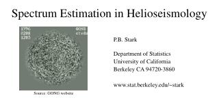
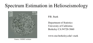
Spectrum Estimation in Helioseismology P.B. Stark Department of Statistics University of California Berkeley CA 94720-3860 www.stat.berkeley.edu/~stark Source: GONG website
Acknowledgements • Most media pirated from websites of • Global Oscillations Network Group (GONG) • Solar and Heliospheric Observer (SOHO) Solar Oscillations Investigation • Collaboration w/ S. Evans (UCB), I.K. Fodor (LLNL), C.R. Genovese (CMU), D.O.Gough (Cambridge), Y. Gu (GONG), R. Komm (GONG), M.J. Thompson (QMW) Source: www.gong.noao.edu Source: sohowww.nascom.nasa.gov
The Difference between Theory and Practice In Theory, there is no difference between Theory and Practice, but in Practice, there is. I’m embarrassed to give a talk about practice to this lofty audience of mathematicians. My first work in helioseismology was theory/methodology for inverse problems. Surprise! Data not K + , {i} iid, zero mean, Var(i) known—but everyone pretends so.
The Sun • Closest star, ~1.5*108km • Radius ~6.96*105 km • Mass ~1.989*1030 kg • Teff ~5780 K • Luminosity ~3.846*1026 J/s • Surface gravity ~274 m/s2 • Age ~4.6*109y • Mean density ~1408 kg/m3 • Z/X ~0.02; Y ~0.24
The Sun Vibrates • Stellar oscillations known since late 1700s. • Sun's oscillation observed in 1960 by Leighton, Noyes, Simon. • Explained as trapped acoustic waves by Ulrich, Leibacher, Stein, 1970-1. Source: SOHO-SOI/MDI website
Pattern is Superposition of Modes • Like vibrations of a spherical guitar string • 3 “quantum numbers” l, m, n • l and m are spherical surface wavenumbers • n is radial wavenumber Source: GONG website
Waves Trapped in Waveguide • Low l modes sample more deeply • p-modes do not sample core well • Sun essentially opaque to EM; transparent to sound & to neutrinos Source: forgotten!
Spectrum is very Regular • Explanation as modes, plus stellar evolutionary theory, predict details of spectrum • Details confirmed in data by Deubner, 1975 Source: GONG
More data for Sun than for Earth • Over 107 modes predicted • Over 250,000 identified • Will be over 106 soon Formal error bars inflated by 200.Hill et al., 1996. Science272, 1292-1295
“5-minute” oscillations • Takes a few hours for energy to travel through the Sun. • p-mode amplitude ~1cm/s • Brightness variation ~10-7 • Last from hours to months • Excited by convection 1 mode 3 modes all modes 40-day time series of mode coefficients, speeded-up by 42,000. l=1, n=20; l=0, 1, 2, 3 A. Kosovichev, SOHO website.
Oscillations Taste Solar Interior • Frequencies sensitive to material properties • Frequencies sensitive to differential rotation • If Sun were spherically symmetric and did not rotate, frequencies of the 2l+1 modes with the same l and n would be equal • Asphericity and rotation break the degeneracy (Scheiner measured 27d equatorial rotation from sunspots by 1630. Polar ~33d.) • Like ultrasound for the Sun
Different Modes sample Sun differently Left: raypath for l=100, n=8 and l=2, n=8 p-modesRight: raypath for l=5, n=10 g-mode. g-modes have not been observed l=20 modes. Left: m=20. Middle: m=16. (Doppler velocities)Right: section through eigenfunction of l=20, m=16, n =14. Gough et al., 1996. Science 272, 1281-1283
Can combine Modes to target locally Cuts through kernels for rotation:A: l=15, m=8. B: l=28, m=14. C: l=28, m=24.D: two targeted combinations: 0.7R, 60o; 0.82R, 30oThompson et al., 1996. Science272, 1300-1305. Estimated rotation rate as a function of depthat three latitudes.Source: SOHO-SOI/MDI website
Goals of Helioseismology • Learn about composition, state, dynamics of closest star: sunspots, heliodynamo, solar cycle • Test/improve theories of stellar evolution • Use Sun as physics lab: conditions unattainable on Earth (neutrino problem, equation of state) • Predict space weather?
Successes so far • Revised depth of the solar convection zone • Ruled out dynamo models with rotation constant on cylinders • Found errors in opacity calculations of numerical nuclear physicists • Progress in solar neutrino problem
Plasma Rivers in the Sun • SOHO “imaged” rivers of solar plasma moving ~10% faster than the surrounding material. • NASA top-10 story, 1997. Source: SOHO SOI/MDI website
Sun Quakes • Can see acoustic waves propagating from a solar flare • Time-distance helioseismology: new field Source: SOHO-SOI/MDI website
Global Oscillations Network Group (GONG) 6-station terrestrial network; Sun never sets Funded by NSF Solar and Heliospheric Observer Solar Oscillations Investigation (SOHO-SOI/MDI) satellite Orbits L1; Sun never sets Funded by NASA and ESA Current Experiments Experiments range from high-resolution to Sun-as-a-star.The most extensive with highest duty cycle are
Velocity from Doppler Shifts: Michelson Doppler Interferometer • Measure amplitudes of 3 light frequencies in Ni I absorption band, 676.8nm • Probes mid-photosphere • Get velocity in each pixel of CCD image • Developed by T. Brown (HAO/NCAR) in 1980's Source: GONG website
Data Reduction Harvey et al., 1996. Science 272, 1284-1286
Why Reduce the Data to Normal Modes? • GONG+ data rate ~4GB/day: can’t invert a year of data Mode parameters are a much smaller set.(N.b. 4GB/day asymptopia) • Identifying mode parameters helps separate the stochastic disturbance from the characteristics of the oscillator • Relationship between the time-domain surface motion of a stochastically excited gaseous ball with magnetic stiffening not well understood
Read tapes from sites. Correct for CCD characteristics Transform intensities to Doppler velocities Calibrate velocities using daily calibration images Find image geometry and modulation transfer function (atmospheric effects, lens dirt, instrument characteristics, ...) High-pass filter to remove steady flows Remap images to heliographic coordinates, interpolate, resample, correct for line-of-sight Transform to spherical harmonics: window, Legendre stack in latitude, FFT in longitude Adjust spherical harmonic coefficients for estimated modulation transfer function Merge time series of spherical harmonic coefficients from different stations; weight for relative uncertainties Fill data gaps of up to 30 minutes by ARMA modeling Compute periodogram of time series of spherical harmonic coefficients Fit parametric model to power spectrum by iterative approximate maximum likelihood Identify quantum numbers; report frequencies, linewidths, background power, and uncertainties GONG Data Pipeline
Steps in Data Processing Raw intensity image Doppler velocity image High-pass filtered to remove rotation & flows
And more steps… Time series of spherical harmonic coefficients Spectra of time series, and fitted parametric models Top: GONG website. Bottom: Hill et al., Science, 1996.
Duty Cycle • Both GONG and SOHO-SOI/MDI try to get uninterrupted data • Other experiments at South Pole—long day • Gaps in data make it harder to estimate the oscillation spectrum: artifacts in periodogram
Effect of Gaps • Don’t observe process of interest. • Observe process × window • Fourier transform of data is FT of process, convolved with FT of window. • FT of window has many large sidelobes • Convolution causes energy to “leak” from distant frequencies into any particular band of interest. 95% duty cycle window Power spectrum of window
Tapering • Want simplicity of periodogram, but less leakage • Traditional approach—multiply data by a smooth “taper” that vanishes where there are no data • Smoother tapersmaller sidelobes, but more local smearing (loss of resolution) • Pose choosing taper as optimization problem
Optimal Tapering • What taper minimizes “leakage” while maximizing resolution? • Leakage is a bias; optimality depends on definition • Broad-band & asymptotic yield eigenvalue problems:
Prolate Spheroidal Tapers • Maximize the fraction of energy in a band [-w, w]around zero • Analytic solution when no gaps: • 2wT tapers nearly perfect • others very poor • Must choose w • Character different with gaps T = 1024, w = 0.004.Fodor&Stark, 2000. IEEE Trans. Sig. Proc., 48, 3472-3483
Minimum Asymptotic Bias Tapers • Minimize integral of spectrum against frequency squared • Leading term in asymptotic bias T = 1024Fodor&Stark, 2000. IEEE Trans. Sig. Proc., 48, 3472-3483
Sine Tapers • Without gaps, approximate minimum asymptotic bias tapers • With gaps, reorthogonalize w.r.t. gap structure T = 1024.Fodor&Stark, 2000. IEEE Trans. Sig. Proc.48, 3472-3483.
Optimization Problems • Prolate and minimum asymptotic bias tapers are top eigenfunctions of large eigenvalue problems • The problems have special structure; can be solved efficiently (top 6 tapers for T=103,680 in < 1day) • Sine tapers very cheap to compute
Sample Concentration of TapersT=1024, w = 0.004 Fodor & Stark, 2000. IEEE Trans. Sig. Proc., 48, 3472-3483
Sample Asymptotic Bias of Tapers, T = 1024 Fodor & Stark, 2000. IEEE Trans. Sig. Proc., 48, 3472-3483
Multitaper Estimation • Top several eigenfunctions have eigenvalues close to 1. • Eigenvalues drop to zero, abruptly for no-gap • Estimates using orthogonal tapers are asymptotically independent (mild conditions) • Averaging spectrum estimates from several “good” tapers can decrease variance without increasing bias much. • Get rank K quadratic estimator.
Multitaper Procedure • Compute K orthogonal tapers, each with good concentration • Multiply data by each taper in turn • Compute periodogram of each product • Average the periodograms Special case: break data into segments
Cheapest is Fine For simulated and real helioseismic time series of length T=103,680, no discernable systematic difference among 12-taper multitaper estimates using the three families of tapers. Use re-orthogonalized sine tapers because they are much cheaper to compute, for each gap pattern in each time series.
Multitaper Simulation • Can combine with segmenting to decrease dependence • Prettier than periodogram; less leakage. • Better, too? T=103,680. Truth in grey. Left panels: periodogram. Right panels: 3-segment 4-taper gapped sine taper estimate. Fodor&Stark, 2000.
Multitaper: SOHO Data • Easier to identify mode parameters from multitaper spectrum • Maximum likelihood more stable; can identify 20% to 60% more modes (Komm et al., 1999. Ap.J., 519, 407-421) SOHO l=85, m=0. T = 103, 680. Periodogram (left) and 3-segment 4 sine taper estimateFodor&Stark, 2000. IEEE Trans. Sig. Proc., 48, 3472-3483
Error bars: Confidence Level in Simulation 1,000 realizations of simulated normal mode data. 95% target confidence level. Fodor & Stark, 2000. IEEE Trans. Sig. Proc., 48, 3472-3483
Pivot • Asymptotic pivot: asymptotic distribution does not depend on unknown parameter • For K multitaper estimate, = 10log10S(f), Pivot: Rn= (T- )/
Depth of Convection Zone • D. O. Gough showed using helioseismic data that the solar convection zone probably is rather thicker than had been thought.
Falsified dynamo models Since the mid-1980s, many studies of solar rotation using frequency splittings (broken degeneracy from rotation) have shed doubt on dynamo models that required rotation to be roughly constant on cylinders in the convection zone.
Errors in Opacity Calculations • The “standard solar model” fit the estimates of soundspeed better with opacity at base of convection zone modified in an ad hoc way. • Physicists who calculated original opacity found bound-state contribution of iron had been underestimated. • Led to 10-20% error in opacity at base of convection zone. • Revised opacities fit solar data • Explained mysterious pulsation period ratios of Cepheid stars Duval, 1984. Nature, 310, p22.
Solar Neutrino Problem • Measurements of solar neutrino flux lower than predicted by nuclear physics + stellar evolution models • Not clear whether problem with nuclear physics or with theory of stellar evolution • Helioseismology suggests low Helium abundance in core not plausible explanation
Linear Inverse Problem for Rotation Assumes eigenfunctions and radial structure known.
Consistency in Linear Inverse Problems • Xi = i + i, i=1, 2, 3, … subset of separable Banach{i} * linear, bounded on {i} iid • consistently estimable w.r.t. weak topology iff{Tk}, Tk Borel function of X1, . . . , Xk s.t. , >0, *, limk P{|Tk - |>} = 0
Importance of Error Distribution • µ a prob. measure on ; µa(B) = µ(B-a), a • Hellinger distance • Pseudo-metric on **: • If restriction to converges uniformly on increasing sequence of compacts to metric compatible with weak topology, and those compacts are totally bdd wrt d, can estimate consistently in weak topology. • For given sequence of functionals {i}, µ rougher consistent estimation easier.
Normal is Hardest Suppose = {: [0,1], T Hilbert} • If {i} iid U[0,1], consistent iff |<i,>|=. • If {i} iid N[0,1], consistent iff |<i,>|2=