Download
1 / 26
280 likes | 488 Vues
Local Helioseismology. Laurent Gizon (Stanford). Outline. Some background Time-distance helioseismology: Solar-cycle variations of large-scale flows Near surface convection Sunspots: structure and dynamics. Why is helioseismology useful?. To test the standard model of stellar structure

E N D
Local Helioseismology Laurent Gizon (Stanford)
Outline • Some background • Time-distance helioseismology: • Solar-cycle variations of large-scale flows • Near surface convection • Sunspots: structure and dynamics
Why is helioseismology useful? • To test the standard model of stellar structure • To help understand solar magnetism
Global modes of resonance Millions of modes of oscillation excited by near-surface turbulent convection. Acoustic modes with similar wave speeds probe similar depths. MDI-SOHO measures Dopplergrams every minute since 1996. Figure: m-averaged medium-l power spectrum (60-day run).
Global p-mode frequency shifts Palle et al. • Frequencies of low-degree acoustic modes of oscillation increase with magnetic activity. • Woodard & Noyes (1985) first notice changes in irradiance oscillation data (ACRIM). • Confirmed by ground-based full-disk velocity data (e.g. Bison). • Fractional change of 2x10⁻⁴ through the solar cycle.
Freq. shifts are localized in latitude microHz medium-l GONG 1D RLS Howe et al. ApJ, 2002 Contours: Kitt Peak magnetic data • Spatially resolved observations: Mt Wilson, GONG, MDI. • Libbrecht & Woodard (1989) showed that frequency shifts must be caused by near-surface perturbations. • The physics of frequency shifts is not understood. We don’t know how to separate magnetic from thermal/density perturbations. • Shifts likely to be caused by magnetic perturbations within 2 Mm of the photosphere (Goldreich, Goode/Dziembowski) or above (Roberts). • Other suggestion: changes in turbulent velocities (Kuhn).
Local helioseismology The goal is to make 3D images of flows, temperature and density inhomogeneities, and magnetic field in the solar interior. Local helioseismology includes different techniques that complement each other (see Gizon & Birch, Living Reviews, submitted). Time-distance helioseismology (Duvall et al. 1993) is based on measurements of travel times for wavepackets travelling between any two points on the solar surface. • Flows along the path break the symmetry between travel times for waves propagating in opposite directions • Travel-time difference flows • Measurements of travel times between all pairs of points give access to the 3D vector flow field, in principle. • Local helioseismology is potentially more powerful than global-mode helioseismology: Longitudinal resolution (3D image) North-south flows
Time-distance diagram (Duvall) Correlation between two surface locations versus distance and time-lag.
Near-surface “global” flows Longitudinal averages from f-mode time-distance helioseismology Rotation Meridional circulation Mean meridional circulation is poleward in both hemispheres (~20 m/s at 20 deg latitude) Important ingredient in some theories of the solar dynamo. Directly observed down to 0.8R, so far (Giles 1998). To study solar-cycle variations: subtract time average over many years… CONFIRMS GLOBAL-MODE HELIOSEISMOLOGY NEW INFORMATION
Meridional circulation vs. depth (Giles 2001) • Inversion of travel times with mass-conservation constraint through the whole convection zone (Giles PhD thesis). • For r/R>0.8 the mean meridional circulation is poleward in both hemispheres and peaks around 25 deg latitude. • The data are consistent with a 3 m/s return flow at the base of the convection zone. Hathaway obtains a similar number from an analysis of sunspot drifts. Fractional radius r/R
Solar-cycle variation of large-scale flows Plots of residuals of rotation and meridional circulation after subtraction of a temporal average. About 50 Mm deep (Beck, Gizon & Duvall, 2002). Zonal flow residuals (torsional oscillations) red=prograde blue= retrograde Increased differential rotation shear at active latitudes. First discovered by Howard & Labonte (1980), agrees with global mode splittings. May be caused by the back reaction of the Lorentz force from a propagating dynamo wave (Schuessler, 1981). [Other explanations exist.] Latitude (deg) Meridional flow residuals Residuals: red=equatorward, green=poleward At 50 Mm depth, residual north-south flow diverging from the mean latitude of activity (agrees with Chou 2001, acoustic imaging). The opposite is seen near the surface! (Gizon 2003, Zhao 2003). Latitude (deg) Year (19962002)
Residuals MC: longitudinal averages • (e) surface inflow (5 m/s) TD/RD • (d) deeper outflow (5 m/s) TD • (a) zonal shear (+/- 5 m/s) TD/RD/Global
Near-surface flows around active regions Local 50 m/s surface flows converging toward active regions (Gizon et al. 2001). Excellent agreement with ring-diagram analysis (Hindman, Gizon et al. 2004). Local inflows responsible for temporal variations of surface meridional flow (Gizon 2004) At depth of 10-15 Mm: an outflow is observed (Haber et al. 2003, Zhao et al. 2003) Looks like a toroidal flow pattern around AR: surface outflow and deeper inflow. Surface inflow consistent with a model by Spruit (2003).
Local flows around AR • Sketch of near-surface flows from local helioseismology. • (a) Zonal shear. (m) meridional flow. • (b) 30-50 m/s large-scale inflow. (c) super-rotation. • Time-distance and ring analyses are consistent (Hindman et al. 2004). • Note that Spruit’s model predicts the inflow.
Convective flows Supergranulation F-mode time-distance (Duvall & Gizon) Spatial sampling = 3 Mm Temporal sampling = 8 hr Horizontal divergence: white = divergent flows black = convergent flows
Wavelike properties of supergranulation The supergranulation pattern appears to propagate in the form of a modulated travelling wave (Gizon, Duvall & Schou, 2003, Nature) The direction of propagation is prograde at the equator, and slightly equatorward of the prograde direction away from the equator. An analysis in Fourier space enables to separate the background advective flows from the non-advective wave speed (65 m/s) Red: advective flow. Green: motion of magnetic features. Dashed: Correlation tracking with 24 hr lag. Supergranulation may be an example of travelling-wave convection. No explanation yet. Although it is likely that the influence of rotation (or rotational shear) on convection is at the origin of this phenomenon (Busse 2003). dt=24hr
Advection of Supergranulation • Flows introduce a Doppler shift in the spectrum. • Shown are the longitudinal averages of zonal and meridional flows in the supergranular layer. • Increased differential rotation shear near AR • North-south residual flow converging toward AR. consistent with near-surface flows from local helioseismology
Sunspot seismology? Complex flow picture. Not always meaningful… Zhao et al. 2003 Gizon et al. 2001
Far side imaging (Lindsey &Braun) From MDI pipeline (almost real time) Predictive power
Linear forward and inverse problemsin local helioseismology Linear sensitivity of travel time to small steady changes in the solar model: In principle, have to consider all possible types ( ) of perturbations, including flows, temperature, density, magnetic field, damping and excitation… A general recipe for computing kernels must include a physical description of the wave field generated by a stochastic source model and the details of the measurement procedure (Gizon & Birch 2002). Linearization is achieved through the Born or Rytov approximations (single-scattering). Done for sound-speed perturbations (Birch et al. 2004). Need to do it for other types of perturbations Still some very hard problems to solve…
P-mode Born sensitivity kernel for sound-speed perturbations (Birch 2004)
Toy problem : sound-speed only (Couvidat et al. 2004) 3D Inversion taking account of correlations in data errors Cut through 3D input sound-speed perturbation 3D Inversion assuming no correlation in data errors • Known input sound speed perturbations • Compute travel times by convolution of (1) with 3D Born kernels. • Add noise to the data with the correct statistics (T=8 hrs). • 3D multi-channel deconvolution
Conclusion Complex flow patterns evolving with the solar cycle in the near-surface shear layer. Are these flows a secondary manifestation of the solar dynamo, or do they play an important role in the organization of solar magnetic fields?