Genetic Algorithm

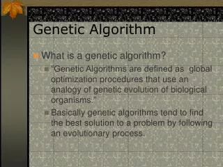
1. Genetic Algorithm Genetic Algorithms (GA) apply an evolutionary approach to inductive learning. GA has been successfully applied to problems that are difficult to solve using conventional techniques such as scheduling problems, traveling salesperson problem, network routing problems and financial marketing.

2. Supervised genetic learning

3. Genetic learning algorithm • Step 1: Initialize a population P of n elements as a potential solution. • Step 2: Until a specified termination condition is satisfied: • 2a: Use a fitness function to evaluate each element of the current solution. If an element passes the fitness criteria, it remains in P. • 2b: The population now contains m elements (m <= n). Use genetic operators to create (n – m) new elements. Add the new elements to the population.

4. Digitalized Genetic knowledge representation • A common technique for representing genetic knowledge is to transform elements into binary strings. • For example, we can represent income range as a string of two bits for assigning “00” to 20-30k, “01” to 30-40k, and “11” to 50-60k.

5. Genetic operator - Crossover • The elements most often used for crossover are those destined to be eliminated from the population. • Crossover forms new elements for the population by combining parts of two elements currently in the population.

6. Genetic operator - Mutation • Mutation is sparingly applied to elements chosen for elimination. • Mutation can be applied by randomly flipping bits (or attribute values) within a single element.

7. Genetic operator - Selection • Selection is to replace to-be-deleted elements by copies of elements that pass the fitness test with high scores. • With selection, the overall fitness of the population is guaranteed to increase.

8. Step 1 of Supervised genetic learning This step initializes a population P of elements. The P referred to population elements. The process modifies the elements of the population until a termination condition is satisfied, which might be all elements of the population meet some minimum criteria. An alternative is a fixed number of iterations of the learning process.

9. Step 2 of supervised genetic learning Step 2a applies a fitness function to evaluate each element currently in the population. With each iteration, elements not satisfying the fitness criteria are eliminated from the population. The final result of a supervised genetic learning session is a set of population elements that best represents the training data.

10. Step 2 of supervised genetic learning Step 2b adds new elements to the population to replace any elements eliminated in step 2a. New elements are formed from previously deleted elements by applying crossover and mutation.

11. An initial population for supervised genetic learning example

12. Question mark in population A question mark in the population means that it is a “don’t care” condition, which implied that the attribute is not important to the learning process.

13. Training Data for Genetic Learning

14. Goal and condition • Our goal is to create a model able to differentiate individuals who have accepted the life insurance promotion from those who have not. • We require that after each iteration of the algorithm, exactly two elements from each class (life insurance promotion=yes) & (life insurance promotion=no) remain in the population.

15. Fitness Function • Let N be the number of matches of the input attribute values of E with training instances from its own class. • Let M be the number of input attribute value matches to all training instances from the competing classes. • Add 1 to M. • Divide N by M. Note: the higher the fitness score, the smaller will be the error rate for the solution.

16. Fitness function for element 1 own class of life insurance promotion = no • Income Range = 20-30k matches with training instances 4 and 5. • No matches for Credit Card Insurance=yes • Sex=Male matches with training instances 5 and 6. • No matches for Age=30-39. • ∴ N = 4

17. Fitness function for element 1 of competing class of life insurance promotion = yes • No matches for Income Range=20-30k • Credit Card Insurance=yes matches with training instance 1. • Sex=Male matches with training instance 1. • Age=30-39 matches with training instances 1 and 3. • ∴M = 4 • ∴F(1) = 4 / 5 = 0.8 • Similarly F(2)=0.86, F(3)=1.2, F(4)=1.0

18. Crossover operation for elements 1 & 2

19. A Second-Generation Population

20. Application of the model(test phase) • To use the model, we can compare a new unknown instance (test data) with the elements of the final population. A simple technique is to give the unknown instance the same classification as the population element to which it is most similar. • The algorithm then randomly chooses one of the m elements and gives the unknown instance the classification of the randomly selected element.

21. Genetic Algorithms & unsupervised Clustering Suppose there are P data instances within the space where each data instance consists of n attribute values. Suppose m clusters are desired. The model will generate k possible solutions. A specific solution contains m n-dimensional points, where each point is a best current representative element for one of the m clusters.

22. For example, S2 represents one of the k possible solutions and contains two elements E21 and E22.

23. Crossover operation A crossover operation is accomplished by moving elements (n-dimensional points) from solution Si to solution Sj. There are several possibilities for implementing mutation operations. One way to mutate solution Si is to swap one or more point coordinates of the elements within Si.

24. Fitness function An applicable fitness function for solution Sj is the average Euclidean distance of the P instances in the n-dimensional space from their closest element within Sj. We take each instance I in P and compute the Enclidean distance from I to each of the m elements in Sj. Lower values represent better fitness scores. Once genetic learning terminates, the best of the k possible solutions is selected as the final solution. Each instance in the n-dimensional space is assigned to the cluster associated with its closest element in the final solution.

25. Training data set for unsupervised GA Instance X Y • 1.0 1.5 • 1.0 4.5 • 2.0 1.5 • 2.0 3.5 • 3.0 2.5 • 5.0 6.0

26. Fitness function for unsupervised GA We apply fitness function to the Training data. We instruct the algorithm to start with a solution set consisting of three plausible solutions (k=3). With m=2, P=6, and k=3, the algorithm generates the initial set of solutions. An element in the solution space contains a single representative data point for each cluster. For example, the data points for solution S1 are (1,0, 1.0) and (5.0,5.0).

27. Euclidean distance Fitness score of d(1.0, 1.0) and d(5.0, 5.0) = min ( Squareroot( |1.0 – 1.0|2 + |1.0 – 1.5|2), Squareroot( |5.0 – 1.0|2 + |5.0 – 1.5|2) + min ( Squareroot( |1.0 – 1.0|2 + |1.0 – 4.5|2), Squareroot( |5.0 – 1.0|2 + |5.0 – 4.5|2) + min ( Squareroot( |1.0 – 2.0|2 + |1.0 – 1.5|2), Squareroot( |5.0 – 2.0|2 + |5.0 – 1.5|2) + min ( Squareroot( |1.0 – 2.0|2 + |1.0 – 3.5|2), Squareroot( |5.0 – 2.0|2 + |5.0 – 3.5|2) + min ( Squareroot( |1.0 – 3.0|2 + |1.0 – 2.5|2), Squareroot( |5.0 – 3.0|2 + |5.0 – 2.5|2) + min ( Squareroot( |1.0 – 5.0|2 + |1.0 – 6.0|2), Squareroot( |5.0 – 5.0|2 + |5.0 – 6.0|2) = 0.5 + 3.5 + 1.11 + 2.69 + 2.5 + 1 = 11.3

28. Solution Population for unsupervised Clustering S1 S2 S3 Solution elements (1.0,1.0) (3.0,2.0) (4.0,3.0) (initial population) (5.0,5.0) (3.0,5.0) (5.0,1.0) Fitness score 11.31 9.78 15.55 ----------------------------------------------------------------------------------------------------------------------------- Solution elements (5.0,1.0) (3.0,2.0) (4.0,3.0) (second generation) (5.0,5.0) (3.0,5.0) (1.0,1.0) Fitness score 17.96 9.78 11.34 ----------------------------------------------------------------------------------------------------------------------------- Solution elements (5.0,5.0) (3.0,2.0) (4.0,3.0) (third generation) (1.0,5.0) (3.0,5.0) (1.0,1.0) Fitness score 13.64 9.78 11.34 -----------------------------------------------------------------------------------------------------------------------------

29. First Generation Solution To compute the fitness score of 11.31 for solution S1 the Euclidean distance between each instance and its closest data point in S1 is summed. To illustrate this, consider instance 1 in training data. The Euclidean distance between (1.0,1.0) and (1.0,1.5) is computed as 0.50. The distance between (5.0,5.0) and (1.0,1.5) is 5.32. The smaller value of 0.50 is represented in the overall fitness score for solution S1. S2 is the best first-generation solution.

30. Second Generation Solution The second generation is obtained by performing a crossover between solutions S1 and S3 with solution element (1.0,1.0) in S1 exchanging places with solution element (5.0,1.0) is S3. The result of the crossover operation improves (decreases) the fitness score for S3 while the score for S1 increases.

31. (Final) Third Generation Solution The third generation is acquired by mutating S1. The mutation interchanges the y-coordinate of the first element in S1 with the x-coordinate of the second element. The mutation results in an improved fitness score for S1. Mutation and crossover continue until a termination condition is satisfied. If the third generation is terminal, then the final solution is S2.

32. Solution for Clustering If S2 (3.0, 2.0) and (3.0, 5.0) is the final solution, then computing the distances between S2 and the following points are: Instances 1, 3 and 5 forming one cluster and instances 2 and 6 forming second cluster, and instance 4 can be in either clusters. Cluster 1 center (3.0, 2.0) Instance X Y 1.0 1.5 2.0 1.5 3.0 2.5 Cluster 2 center (3.0, 5.0) Instance X Y 1.0 4.5 2.0 3.5 5.0 6.0

33. General considerations for GA • GA are designed to find globally optimized solutions. • The fitness function determines the computation complexity of a genetic algorithm. • GA explain their results to the extent that the fitness function is understandable. • Transforming the data to a form suitable for a genetic algorithm can be a challenge.

34. Choosing a data mining technique Given a set of data containing attributes and values to be mined together with information about the nature of the data and the problem to be solved, determine an appropriate data mining technique.

35. Considerations for choosing data mining techniques • Is learning supervised or unsupervised? • Do we require a clear explanation about the relationships present in the data? • Is there one set of input attributes and one set of output attributes or can attributes interact with one another in several ways? • Is the input data categorical, numeric, or a combination of both? • If learning is supervised, is there one output attribute or are there several output attributes? Are the output attribute(s) categorical or numeric?

36. Behavior of different data mining techniques • Neural networks is black-box structured, and is a poor choice if an explanation about what has been learned is required. • Association rule is a best choice when attributes are allowed to play multiple roles in the data mining process. • Decision trees can determine attributes most predictive of class membership. • Neural networks and clustering assume attributes to be of equal importance. • Neural networks tend to outperform other models when a wealth of noisy data are present. • Algorithms for building decision trees typically execute faster than neural network or genetic learning. • Genetic algorithms is typically used for problems that cannot be solved with traditional techniques.

37. Review question 10 Given the following training data set Training instance Income range Credit card insurance Sex Age 1 30-40k Yes Male 30-39 2 30-40k No Female 40-49 3 50-60k No Female 30-39 4 20-30k No Female 50-59 5 20-30k No Male 20-29 6 30-40k No Male 40-49 Describe the steps needed to apply unsupervised genetic learning to cluster the instances of the credit card promotion database.

38. Tutorial Question 10 Given the following training data set Training instance Income range Credit card insurance Sex Age 1 30-40k Yes Male 30-39 2 30-40k No Female 40-49 3 50-60k No Female 30-39 4 20-30k No Female 50-59 5 20-30k No Male 20-29 6 30-40k No Male 40-49 After transforming the input data into numeric such as yes=1, no=2, male=1, female=2, 20-29=1, 30-39=2, 40-49=3, 50-59=4, 20-30k=1, 30-40k=2, 40-50k=3, 50-60k=4, the training data set becomes: T(1)=(2,1,1,2) T(2)=(2,2,2,3) T(3)=(4,2,2,2) T(4)=(1,2,2,4) T(5)=(1,2,1,1) T(6)=(2,2,1,3) Assume there are two set of initial population for two clusters as: Solution 1 of 2 clusters centers: K1(1,1,1,1), (4,2,2,4) Solution 2 of 2 clusters centers: K2(4,4,4,4), (2,2,1,1) Choose the best solution based on their fitness function score by use of unsupervised genetic learning.

39. Reading assignment “Data Mining: A Tutorial-based Primer” by Richard J Roiger and Michael W. Geatz, published by Person Education in 2003, pp.89-101.