Genetic Algorithm
Genetic Algorithm. Outline. Evolutionary Computation Genetic algorithms Genetic Programming. 緣起. 達爾文 (Charles Darwin) 生於英國 1809/02/12 物種原始 (1859) 理論 (Natural selection)

Genetic Algorithm
E N D
Presentation Transcript
Outline • Evolutionary Computation • Genetic algorithms • Genetic Programming
緣起 • 達爾文(Charles Darwin) • 生於英國1809/02/12 • 物種原始(1859) • 理論(Natural selection) • 物種隨環境的變動而改變 • 生物演化為連續性的漸變 • 同一類生物來自共同的祖先 • 適者生存,不適者淘汰(天擇說)
Evolution Strategies 20世紀50年代即有生物學家以電腦(計算機)模擬生物的遺傳現象。 • 源起 • RechenbegandSchwefel(1965) (Evolution Strategies) • 1965年,德國人Rechenbergand Schwefel在柏林工業大學(the Technical University of Berlin),為了解決流體力學中,模型控制裏實數參數最佳化的問題。合作發明了一種新的方法運用電腦以求解決問題,就是「演化策略」(Evolution Strategies) • 根據生物演化的現象,Rechenberg歸納以下的結論:『演化會使生物過程達到最佳化,而演化本身也是一種生物過程,所以演化必然使本身也達到最佳化。』這種探討關於演化本身的演化,也就是考慮到演化的策略 • 提出以突變(mutate)為主的演化方法
Genetic Algorithm • 同時 • J. H. Holland(University of Michigan) • 1967年美國芝加哥大學J.H.Holland教授及其學生、同僚,發展了一套"適應系統"的進化演算。 • 1968年提出模式理論。 • 1975年出版“自然界和人工系統的適應性(Adaptation in Nature and Artificial System) (書:代表作) ,發展了遺傳演算法的理論基礎 • 介紹了交配(Crossover)遺傳運算
Evolutionary Programming • Proposed by L. J. Fogelin 1966 and refined by his son D.B. Fogelin 1991 • The goal of EP is to achieve intelligent behaviorthrough simulated evolution • L. Fogel想要發展和人工智能中專家系統不同的模型,以便消除系統對人為設計的依賴,而能自我調適。由演化的觀點出發,他將智能視為一種天擇的產物。所以不像專家系統需要模擬人類的思考行為,而是直接讓系統演化出所須的行為模式。 • Genetic Programming Proposed by J. R. Koza in 1992 • Genetic Algorithms, Genetic Programming, Evolution Strategies, and Evolutionary Programming ,共同成為Evolutionary Computation 最重要的四大分支
Evolutionary Algorithms Evolutionary Algorithms Genetic Algorithms (GA) Genetic Programming (GP) Evolution Strategies (ES) Evolutionary Programming (EP)
Problem solution using evolutionary algorithms Coding of solutions Objective function Genetic search problem solution Genetic operators Specific knowledge Fitness assignment selection Genetic search mutation replication Recombination crossover
ES、EP generation reproduction Genetic operators selection generation
GAs Simple Genetic Algorithm() { Initialize population; evaluate population; while (termination criterion not reached) { select solutions for next population (reproduction); perform crossover and mutation; evaluate population; } }
Basics of GAs • A genetic algorithm is a search procedure based on the mechanics of natural selection and genetics. • Algorithm starts with a set of solutions (represented by chromosomes) calledpopulation. Solutions from one population are taken and used to form a new population. • This is motivated by a hope, that the new population will be better than the old one. • Solutions which are selected to form new solutions (offspring) are selected according to their fitness - the more suitable they are, the more chances they are reproduced. • This is repeated until some condition (for example number of populations or improvement of the best solution) is satisfied. • Require two things Survival-of-the-fittest Variation
2 important genetic operators • Crossover • Mutation
Single point crossover parent 0|0|0|0|0|0|0|0|0|0|0|0|0|0|0|0 1|1|1|1|1|1|1|1|1|1|1|1|1|1|1|1 Drawback: position bias Gene in loci 1 and 2 often Crossover together children |0|0|0|0|0|0|0|0|0|0|0|0|0 1|1|1 0|0|0 |1|1|1|1|1|1|1|1|1|1|1|1|1
Multipoint crossover parent 0|0|0|0|0|0|0|0|0|0|0|0|0|0|0|0 1|1|1|1|1|1|1|1|1|1|1|1|1|1|1|1 children 1|1|1|1|1 1|1 0|0|0|0 ||0|0|0|0|0 1|1|1|1 ||1|1|1|1|1| 0|0|0|0|0 |0|0
Uniform crossover parent 0|0|0|0|0|0|0|0|0|0|0|0|0|0|0|0 1|1|1|1|1|1|1|1|1|1|1|1|1|1|1|1 children each parent 50% 0|1|0|0|1|1|0|0|1|0|1|1|0|0|1|0 1|0|1|1|0|0|1|1|0|1|0|0|1|1|0|1 Inverse of the other child
Point mutate parent 0|1|0|0|1|1|0|0|1|0|1|1|0|0|1|0 child 0|1|0|0|1|1|0|0|1|0|1|0|0|0|1|0
Crossover for real-valued variables • The original GA was designed for binary-encoded data Single arithmetic crossover (x1, x2, …, xn) (y1, y2,…,yn) α (y1,y2,…,αxk+(1-α)yk,…,yn) Ex: (0.5,1.0,1.5,2.0) (0.2,0.7, 0.2, 0.7) (x1,x2,…,αyk+(1-α)xk,…,xn) At 3nd gene α=0.4 (0.2,0.7,(0.4)(1.5)+(0.6)(0.2),0.7) (0.5,1.0,(0.4)(0.2)+(0.6)(1.5), 2.0) (0.5,1.0,0.98,2.0) (0.2,0.7,0.72,0.7)
Simple arithmetic crossover (x1, x2, …, xn) (y1, y2,…,yn) (x1, x2,…, α yk+(1- α)xk,…, α yn+(1- α)xn) (y1, y2, …, α xk+(1- α)yk,…, α xn+(1- α)yn)
Discrete Crossover: each gene is chosen with uniform probability to be the gene of one or the other of the parents’ chromosomes Parents : (0.5, 1.0, 1.5,2.0), (0.2,0.7, 0.2, 0.7) Child: (0.2, 0.7, 1.5, 0.7)
Normally distributed mutation Random shock may be added to each variable. The shock Should be normally distributed N(0,σ) Pm =1, each variable is mutated Suppose the shock is N(µ=0, σ=0.1) Shock are 0.05, -0.17, -0.03, 0.08 Chromosome (0.2,0.7,1.5, 0.7) is mutated to (0.2+0.05, 0.7-0.17, 1.5-0.03, 0.7+0.08) = (0.25, 0.53, 1.47, 0.78)
A simple GA at work • EncodeEncode solutions to a problem as a set of numbers. • Define a Fitness MetricThis is a number that defines a solution's “goodness”. • EvolveImprove the population by a process of Darwinian selection favoring the reproduction of fitter solutions. • Initialize population by randomly generating N genomes. • Evaluate fitness of all the individuals in the population. • Repeat this loop until the solutions are adequate.
Find the maximum of N(µ=16,σ=4) • 最大值x=16,假設不知道! f(x) Init: pc=0.75, pm=0.002 Representation: n=4 l=5 00000-11111 (0) (31) x 4 8 12 16 20 24 28
4 init. chromosomes 00100 (4), 01001(9), 11011(27) and 11111(31) Fitness fu. = f(x)
Selection probability chromosome Decimal value fitness 0.04425 4 0.001108 00100 01001 9 0.021569 0.86145 11011 27 0.002273 0.09078 11111 31 0.000088 0.00351
selection : 01001, 11011 are selected • Crossover: at the second bit parent 0 1 0 0 1 1 1 0 1 1 No mutate this time children 0 1 0 1 1 1 1 0 0 1 11 25
selection : 01001, 00100 are selected • No crossover this time New population: 00100, 01001, 01011(11), 11001 11 is a closer to 16!
Selection probability chromosome Decimal value fitness 0.014527 4 0.001108 00100 01001 9 0.021569 0.282783 01011 11 0.045662 0.598657 0.104003 11001 25 0.000088
selection • At 1st generation, 01001(9) dominated the fitness measure (86%), it will be selected too many times, generates too many copies, which impairs GA search capability (easy to stuck at local optimum)---crowding phenomenon • Variability vs fitness
Selection (contd) • Boltzmann selection T: temperature, from high to low At the beginning, fitness bias is suppressed, so variability is high, the search space is large At the end, fitness bias is enlarged, so global optimum is found quickly.
Elitism: requires Gas to retain a certain number of the fittest chromosomes. • Ranking: ranks the chromosomes according to their fitness, reduces crowding problem, but low variability • Etc.
Advantages of GA • GAs can search spaces of hypotheses containing complex interacting parts, where the impact of each part on overall hypothesis fitness may be difficult to model • GAs are easily parallelized and can take advantage of the decreasing costs of powerful computer hardware