Download

1 / 11
140 likes | 301 Vues
Finite Element Primer for Engineers: Part 2 Mike Barton & S. D. Rajan. Introduction to the Finite Element Method (FEM) Steps in Using the FEM (an Example from Solid Mechanics) Examples Commercial FEM Software Competing Technologies Future Trends Internet Resources References. Contents.

E N D
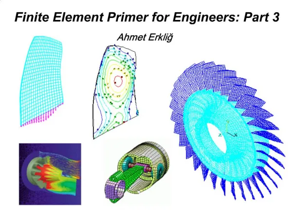
Finite Element Primer for Engineers: Part 2 Mike Barton & S. D. Rajan
Introduction to the Finite Element Method (FEM) Steps in Using the FEM (an Example from Solid Mechanics) Examples Commercial FEM Software Competing Technologies Future Trends Internet Resources References Contents
A FEM model in solid mechanics can be thought of as a system of assembled springs. When a load is applied, all elements deform until all forces balance. F = Kd K is dependant upon Young’s modulus and Poisson’s ratio, as well as the geometry. Equations from discrete elements are assembled together to form the global stiffness matrix. Deflections are obtained by solving the assembled set of linear equations. Stresses and strains are calculated from the deflections. dxi 1 dxi 2 2 dyi 1 1 dyi 2 4 3 FEM Applied to Solid Mechanics Problems Create elements of the beam Nodal displacement and forces
Classification of Solid-Mechanics Problems Analysis of solids Dynamics Static Advanced Elementary Stress Stiffening Behavior of Solids Large Displacement Geometric Instability Linear Nonlinear Fracture Plasticity Material Viscoplasticity Geometric Classification of solids Skeletal Systems 1D Elements Plates and Shells 2D Elements Solid Blocks 3D Elements Plane Stress Plane Strain Axisymmetric Plate Bending Shells with flat elements Shells with curved elements Trusses Cables Pipes Brick Elements Tetrahedral Elements General Elements
[K] {u} = {Fapp} + {Fth} + {Fpr} + {Fma} + {Fpl} + {Fcr} + {Fsw} + {Fld} [K] = total stiffness matrix {u} = nodal displacement {Fapp} = applied nodal force load vector {Fth} = applied element thermal load vector {Fpr} = applied element pressure load vector {Fma} = applied element body force vector {Fpl} = element plastic strain load vector {Fcr} = element creep strain load vector {Fsw} = element swelling strain load vector {Fld} = element large deflection load vector Governing Equation for Solid Mechanics Problems • Basic equation for a static analysis is as follows:
Step 1 - Discretization: The problem domain is discretized into a collection of simple shapes, or elements. Step 2 - Develop Element Equations: Developed using the physics of the problem, and typically Galerkin’s Method or variational principles. Step 3 - Assembly: The element equations for each element in the FEM mesh are assembled into a set of global equations that model the properties of the entire system. Step 4 - Application of Boundary Conditions: Solution cannot be obtained unless boundary conditions are applied. They reflect the known values for certain primary unknowns. Imposing the boundary conditions modifies the global equations. Step 5 - Solve for Primary Unknowns: The modified global equations are solved for the primary unknowns at the nodes. Step 6 - Calculate Derived Variables: Calculated using the nodal values of the primary variables. Six Steps in the Finite Element Method
Process Flow in a Typical FEM Analysis Problem Definition Analysis and design decisions Stop Start • Pre-processor • Reads or generates nodes and elements (ex: ANSYS) • Reads or generates material property data. • Reads or generates boundary conditions (loads and constraints.) • Processor • Generates element shape functions • Calculates master element equations • Calculates transformation matrices • Maps element equations into global system • Assembles element equations • Introduces boundary conditions • Performs solution procedures • Post-processor • Prints or plots contours of stress components. • Prints or plots contours of displacements. • Evaluates and prints error bounds. Step 6 Step 1, Step 4 Steps 2, 3, 5
Step 1: Discretization - Mesh Generation surface model airfoil geometry (from CAD program) mesh generator ET,1,SOLID45 N, 1, 183.894081 , -.770218637 , 5.30522740 N, 2, 183.893935 , -.838009645 , 5.29452965 . . TYPE, 1 E, 1, 2, 80, 79, 4, 5, 83, 82 E, 2, 3, 81, 80, 5, 6, 84, 83 . . . meshed model
DisplacementsDOF constraints usually specified at model boundaries to define rigid supports. Forces and MomentsConcentrated loads on nodes usually specified on the model exterior. PressuresSurface loads usually specified on the model exterior. TemperaturesInput at nodes to study the effect of thermal expansion or contraction. Inertia LoadsLoads that affect the entire structure (ex: acceleration, rotation). Step 4: Boundary Conditions for a Solid Mechanics Problem
Step 4: Applying Boundary Conditions (Thermal Loads) Nodes from FE Modeler bf, 1,temp, 149.77 bf, 2,temp, 149.78 . . . bf, 1637,temp, 303.64 bf, 1638,temp, 303.63 Temp mapper Thermal Soln Files
Speed, temperature and hub fixity applied to sample problem. FE Modeler used to apply speed and hub constraint. Step 4: Applying Boundary Conditions (Other Loads) antype,static omega,10400*3.1416/30 d,1,all,0,0,57,1