Interactive Shortest Path
Interactive Shortest Path. A n Image Segmentation Technique. Jonathan-Lee Jones. Overview. Dijkstra’s Shortest Path User Interaction – Hard and Soft Input The Energy Function A Multi-Layer Approach Examples Problems and Queries. Dijkstra’s Shortest PAth.


Interactive Shortest Path
E N D
Presentation Transcript
Interactive Shortest Path An Image Segmentation Technique Jonathan-Lee Jones
Overview • Dijkstra’s Shortest Path • User Interaction – Hard and Soft Input • The Energy Function • A Multi-Layer Approach • Examples • Problems and Queries
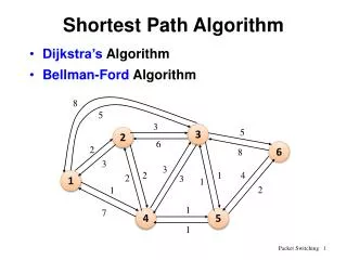
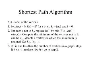
Dijkstra’s Shortest PAth • Dijkstra’s is a shortest path algorithm for non negative weighted edges that generates a shortest path tree. • For a given source vertex (node) in the graph, the algorithm finds the path with lowest cost (i.e. the shortest path) between that vertex and every other vertex • It is of the order O(|V|)2where V is the number of vertices.
User Interaction – Hard Input • In a Hard User Input Paradigm the user labelled points or areas are assigned to either background or foreground (in the case of graph cut for example), or set as fixed points that the path must go through (in the case of shortest path algorithms). This requires the user give very precise input.
User Interaction – Soft Input • In a Soft User Input Paradigm the user labelled points are used as elastic attraction points. These exhibit a tendency to pull the selection towards them, but the shortest path does not necessarily move through them all. In this way user input needs be less precise.
The Energy Function Unfortunately, in its current form the problem cannot be solved efficiently. The third term is devoted to the attraction points. The first is an attraction to image edges, realized by some edge detector g which assigns low cost to high image gradients. The second term penalizes the curvature of the curve and hence favors smooth curves.
The Energy Function • For the specific case of λ = 0 and g(y) = 1 and α → ∞ (i.e. α sufficiently large), the problem amounts to finding the shortest path connecting all attractor points. This problem is known as the Euclidean Traveling Salesman Problem and was shown to be NP-hard
Euclidean Travelling Salesman Problem • The most direct solution would be to try all permutations (ordered combinations) and see which one is cheapest (using brute force search). The running time for this approach lies within a polynomial factor of , the factorial of the number of cities, so this solution becomes impractical even for only 20 cities.
Solving the Problem • Fortunately it turns out that the problem becomes solvable if we impose the set of attraction points to be ordered. • The order is now imposed by enforcing the constraints
A Multi-Layer Approach For each input point Xi we add an additional layer as a copy of the image to the graph. Thus we have K + 1 layers and each pixel p corresponds to K + 1 nodes vp,1 , . . . , vp,K +1 .
Intra-Layer Edges Edges within each copy of the image plane favoring paths along strong gradient edges. Weights are set according to the edge detector function g.
Inter-Layer Edges Edges between copies of the image favor transitions in the vicinity of the attraction points. Edge weights are set according to the distance between input point X and pixel v. The attraction point defines circles on the plane where the transition edges have equal costs.
Problems and Queries • Problems with the method as described • In the method described in the paper, all pixels on the top layer are connected to the source, and the bottom layer to the sync. There are no express start and stop points mentioned, so in the example in their paper, I cannot see why the shortest path wouldn’t start at the first user point.
Problems and Queries • Problems with the method as described • In the diagram from the paper, there are 2 labelled user points, X1 and X2 • Why would the shortest path go from the labelled green dots (not user points) if they were distinctly labelled?
Problems and Queries • The more user points, the slower it becomes. • As more user input is added, a new layer is created every time. • This increases the complexity of the graph with every point. • Paradoxically, the more user input (help) is given, the slower the system becomes. Take a 1000 x 1000 image That give V =16,000,000 for 1 layer. With n user points… V = 17,000,000 x (n+1)