Download
1 / 6
60 likes | 136 Vues
Explore aftershocks induced by earthquake stress in Joshua Tree, CA, visualized through seismic data. Discover how Interferometric SAR revolutionizes earthquake studies and other applications worldwide.

E N D
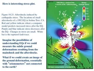
Here is interesting stress plot. Figure 10.21: Aftershocks induced by earthquake stress. The locations of small aftershocks of a 1992 EQ in Joshua Tree, CA. Red and yellow indicate where a computer model predicts increased stress after the EQ. Purple and blue indicate stress decreases after the EQ. Changes in stress are small. White bar is the ruptured fault trace. Imagine the possibilities of understanding EQs if we could measure the subtle ground deformations resulting from the mainshock and the aftershocks. What if we could create an image of the ground deformation, essentially with “seismometers” not connected to the earth?
This is the Landers EQ in CA. June 28th, 1992. A right lateral strike slip fault. This radar interferogram depicts motion occurring during the 1992 Landers earthquake in southern California. These data were acquired by the ERS-1 satellite in orbit 500 miles above the earth, and cover an area approximately 30 by 50 miles in size. Each color "fringe" represents 2.8 cm of ground deformation that occurred during the earthquake, and shows how the Earth's crust readjusted itself to a new distribution of forces along the fault (shown in black) when the earthquake struck. figure not in book
Observed interferogram calculated from ERS-1 SAR images taken before (April 24, 1992) and after (June 18, 1993) the earthquake. Each fringe denotes 28 mm of change in range. The number of fringes increases from zero at the northern edge of the image, where no coseismic displacement is assumed, to at least 20, representing 560 mm in range difference, in the cores of the lobes adjacent to the fault. The asymmetry between the two sides of the fault is due to the curvature of the fault. The spatial distribution is key. Imagine being able to monitor subtle, aseismic ground deformation – a map of stress built-up over time. Locations along known faults where stress is accumulating might be expected to rupture before other locations where aseismic strain is not accumulating. figure not in book
New findings indicate that more than half of the right-lateral motion of the Eastern California shear zone is sharply concentrated along the Blackwater Little Lake fault system. The rapid strain accumulation observed along the fault system indicates that the fault is building up stress in the shallow crust at a rate three times faster than the rate inferred from geological observations. This may be the manifestation of stress transfer between the Garlock fault and other faults in the Mojave area, in particular those that produced the magnitude 7.3 Landers earthquake in 1992 and the magnitude 7.8 Owens Valley earthquake in 1872. figure not in book
Interferometric SAR • Revolutionizing the study of earthquakes by densifying the spatial distribution of measurements, and with a high spatial resolution. • Also Used In: • Glacier velocity and mass balance studies • Groundwater withdrawal and injection • Floodplain water storage changes and flow hydraulics • Construction of a global high resolution topographic data set (SRTM) • Atmospheric water vapor studies • And more…