Download
1 / 22
220 likes | 262 Vues
Explore the fusion of model & data in carbon-water systems using Ensemble Kalman Filter. Learn about Australian Water Availability Project & OptIC project. Understand target variables, cost function, fusion methods & more. Develop a Hydrological and Terrestrial Biosphere Data Assimilation System for Australia. Conduct analysis, drought assessments, and national water balance. Model includes soil moisture, leaf carbon, water fluxes, and carbon fluxes.

E N D
Model-data fusion for the coupled carbon-water system Cathy Trudinger, Michael Raupach, Peter BriggsCSIRO Marine and Atmospheric Research, Australia and Peter RaynerLSCE, France Email: cathy.trudinger@csiro.au
Outline • Model-data fusion (= data assimilation + parameter estimation) • Parameter estimation with the Kalman filter • Australian Water Availability Project • OptIC project – Optimisation Intercomparison
Model-data fusion Observations:- ‘Real world’ representation- Incomplete, patchy- No forecast capability Model:- Process representation- Subjective, incomplete- Capable of interpolation & forecast Fusion:Optimal combination(involves model-obs mismatch & strategy to minimise) Analysis:- “Best of both worlds”- Identify model weaknesses- Forecast capability - Confidence limits
Choices in model-data fusion • Target variables – what model quantities to vary to match observations – e.g. initial conditions, model parameters, time-varying model quantities, forcing • Cost function – measure of misfit between observations and corresponding model quantitiese.g. J(targets) = (H(targets) - obs)2 + (targets - priors)2 • Fusion method - search strategy • Batch (non-sequential) e.g. down-gradient, global search • Sequential e.g. Kalman filter Approach and issues will differ to some extent between disciplines – e.g. numerical weather prediction vs terrestrial carbon cycle
The Ensemble Kalman filter • Ensemble Kalman filter (EnKF) – sequential method that uses Monte Carlo techniques; error statistics are represented using an ensemble of model states. • Two steps: • Model used to predict from one time to next • Update using observation Initialensemble Update using measurement Time: t0 t1 t2 Model predicts
Parameter estimation with the Ensemble Kalman filter • Augmented state vector to be estimated contains • Time-dependent model variables • Time-independent model parameters • State vector estimate at any time is due to observations up to that time
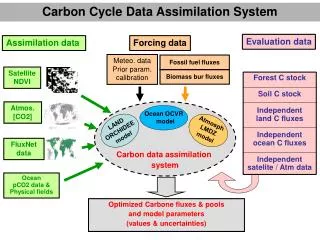
Our component of Australian Water Availability project: develop a Hydrological and Terrestrial Biosphere Data Assimilation System for Australia MODEL • Soil moisture • Leaf carbon • Water fluxes • Carbon fluxes OBSERVATIONS • NDVI • Monthly river flows • Weather: rainfall, solar radiation, temperature PRIOR INFORMATION • Initial parameter estimates • Soil, vegetation types MODEL-DATA FUSION • Ensemble Kalman Filter • Down-gradient method (LM) • Analysis of past, present and future water and carbon budgets • Maps of soil moisture, vegetation growth • Process understanding • Drought assessments, national water balance
AWAP- Dynamic Model and Observation Model Timestep = 1 daySpatial resolution = 5x5 km • State variables (x) and dynamic model • Dynamic model is of general form dx/dt = F (x, u, p) • All fluxes (F) are functions F (x, u, p) = F (state vector, met forcing, params) • Governing equations for state vector x = (W, CL): Soil water W: Leaf carbon CL: • Observations (z) and observation model • NDVI = func(CL) • Catchment discharge = average of FWR + FWD [- extraction- river loss] • State vector in EnKF: x = [W, CL, NDVI, Dis, params]
Southern Murray Darling Basin, Australia:"unimpaired" gauged catchments
J F M A M J J A S O N D 81 82 Murrumbidgee Relative Soil Moisture (0 to 1) 83 84 85 86 87 88 89 90 91 92 93 94 95 96 97 98 99 00 01 (Forward run with priors, no assimilation) 02 03 04 05
Predicted and observed discharge 11 unimpaired catchments in Murrumbidgee basin 25-year time series: Jan 1981 to December 2005 (Forward run with priors, no assimilation)
Model-data synthesis approach:- State and parameter estimation with the EnKF- Assimilate NDVI and monthly catchment discharge Why Kalman filter?- Can account for model error (stochastic component)- Consistent statistics (uncertainty analysis) - Forecast capability (with uncertainty) • Issues:- Time-averaged observations in EnKF (e.g. monthly catchment discharge)- Specifying statistical model (model and observation errors) - KF (sequential) vs batch parameter estimation methods? (using Levenberg-Marquardt method; also OptIC project)
Estimated parameters Preliminary results: Adelong Creek Blue = Ensemble Kalman filter (sequential) Red = Levenberg-Marquardt (PEST) (batch) Monthly mean discharge/runoff
OptIC project Optimisation method intercomparison • International intercomparison of parameter estimation methods in biogeochemistry • Simple test model, noisy pseudo-data • 9 participants submitted results • Methods used: • Down-gradient (Levenberg-Marquardt, adjoint), • Sequential (extended Kalman filter, ensemble Kalman filter) • Global search (Metropolis, Metropolis MCMC, Metropolis-Hastings MCMC).
OptIC model Estimate parameters p1, p2, k1, k2 whereF(t) – forcing (log-Markovian i.e. log of forcing is Markovian) x1 – fast storex2 – slow storep1, p2 – scales for effect of x1 and x2 limitation of productionk1, k2 – decay rates for poolss0 – seed production (constant value to prevent collapse)
Noisy pseudo-observations T1: Gaussian (G) T4: Gaussian but noise in x2 correlated with noise in x1 (GC) T6: Gaussian with 99% of x2 data missing (GM) T2: Log-normal (L) T3: Gaussian + temporally correlated (Markov) (GT) T5: Gaussian + drifts (GD)
Estimates divided by true parameters p1 p2 k1 k2
Cost function Some participants used cost functions with weights, wi(t), that depended on each noisy observation zi(t)
Down-gradient KF Global-search wi(t) = f(zi(t)) less successful than constant weights
Choice of cost function • Evans (2003) – review of parameter estimation in biogeochemical models - “it was hard to find two groups of workers who made the same choice for the form of the misfit function”, with most of the differences being in the form of the weights. • Evans (2003) and the OptIC project emphasise that the choice of cost function matters, and should be made deliberately not by accident or default. (Evans 2003, J. Marine Systems)
Optic project results • Choice of cost function had large impact on results • Most troublesome noise types:- temporally correlated noise • The Kalman filter did as well as the batch methods • For more information on OptIc:http://www.globalcarbonproject.org/ACTIVITIES/OptIC.htm