Download
1 / 37
370 likes | 493 Vues
Understanding the carbon cycle of forest ecosystems: a model-data fusion approach. Mathew Williams School of GeoSciences, University of Edinburgh. Overview. Problems with assessing forest C dynamics Model-data fusion Process dynamics Spatial variability and scaling. Eddy fluxes.

E N D
Understanding the carbon cycle of forest ecosystems: a model-data fusion approach Mathew Williams School of GeoSciences, University of Edinburgh
Overview • Problems with assessing forest C dynamics • Model-data fusion • Process dynamics • Spatial variability and scaling
Eddy fluxes Leaf chamber Soil chamber Litter traps CO2 ATMOSPHERE Carbon flow Photosynthesis Autotrophic Respiration Heterotrophic respiration Leaves Litterfall Stems Translocation Litter Roots Soil biota Decomposition Soil organic matter
Modelling C exchanges Af Lf Cfoliage Rh Ra Ar Lr GPP Croot Clitter D Aw Lw Cwood CSOM/CWD
Senescence & disturbance Photosynthesis & plant respiration Phenology & allocation Microbial & soil processes Af Lf Cfoliage Rh Ra Ar Lr GPP Croot Clitter D Climate drivers Aw Lw Cwood CSOM/CWD Non linear functions of temperature Feedback from Cf Simple linear functions
FUSION ANALYSIS ANALYSIS + Complete + Clear confidence limits + Capable of forecasts Improving estimates of C dynamics MODELS MODELS + Capable of interpolation & forecasts - Subjective & inaccurate? OBSERVATIONS +Clear confidence limits - Incomplete, patchy - Net fluxes OBSERVATIONS
Combining models and observations • Are observations consistent among themselves and with the model? • What processes are constrained by observations? • Can multiple constraints improve analyses? • State estimation with EnKF • REFLEX experiment
MDF: The Kalman Filter Initial state Drivers Forecast Observations Predictions At Ft+1 Dt+1 F´t+1 MODEL OPERATOR P Assimilation At+1 Analysis
Observations – Ponderosa Pine, OR (Bev Law) Flux tower (2000-2) Sap flow Soil/stem/leaf respiration LAI, stem, root biomass Litter fall measurements
= observation — = mean analysis | = SD of the analysis Time (days since 1 Jan 2000) Williams et al GCB (2005)
= observation — = mean analysis | = SD of the analysis Time (days since 1 Jan 2000) Williams et al GCB (2005)
Data brings confidence =observation — = mean analysis | = SD of the analysis Williams et al, GCB (2005)
Outstanding questions • Are the confidence intervals generated by MDF reliable? • How do different MDF approaches compare? • How can model error be characterised? • Can MDF produce reliable estimates of model parameters consistent with observations?
Reflex experiment • Objectives: To compare the strengths and weaknesses of various model-data fusion techniques for estimating carbon model parameters and predicting carbon fluxes. • Real and synthetic observations from evergreen and deciduous ecosystems • Evergreen and deciduous models • Multiple MDF techniques www.carbonfusion.org
Model and parameters Ra Atolab Clab Afromlab Lf Cf Rh1 Rh2 Af Ar Lr GPP Cr Clit D Aw Lw Cw CSOM
Parameter constraint Consistency among methods Confidence intervals constrained by the data Consistent with known “truth” “truth”
Parameter summary • Parameters closely associated with foliage and gas exchange are better constrained • Parameters for wood and roots poorly constrained and even biased • Similar parameter consistency values for synthetic and true data • Correlated parameters were neither better nor worse constrained
Re GPP NEE Confidence interval (gC m-2 yr-1) Fraction of successful annual flux tests (3 years x 2 sites, n=6) Testing algorithms – synthetic data Synthetic data
State retrieval summary • Confidence interval estimates differed widely • Some techniques balanced success with narrow confidence intervals • Some techniques allowed large slow pools to diverge unrealistically • Decomposition of NEE into GPP/Re was generally successful using daily data • Model error = 88% • Prediction error = 31%
Height of sensor and field of view 3.0 m 2.0 m 1.5 m 1.0 m 0.5 m 0.2 m 4.5 m 3.0 m 2.35 m 1.5 m 0.75 m 0.1 m
A multiscale experimental design macroscale microscale Distance (m) Distance (m) (Williams et al. 2008)
Linear averaged Skye NDVIs (collected at 0.2 x 02 m resolution with diffuser off) versus measured NDVIs at coarser spatial scales with diffuser on
Relationships between estimated LAI (using both Skye NDVI and LI-COR LAI-2000 observations at 0.2 m resolution, linearly averaged for upscaling) versus Skye NDVI at different spatial scales.
Frequency histograms for LAI estimates in the microscale site at a range of resolutions. (Williams et al. 2008)
Ground EO Ground + EO Error (Williams et al. 2008)
Spatial analysis summary • Scale invariance in LAI-NDVI relationships at scales > vegetation patches • However spatial variability is high so Kriging has limited usefulness • Over scales >50 m interpolation error was of similar magnitude to the uncertainty in the Landsat NDVI calibration to LAI • Characterisation of spatial LAI errors provides key data for spatial data assimilation
Conclusions • Model data fusion provides insights into information retrieval from noisy and incomplete observations • Challenges and opportunities: • Linking to observations of C pools, tree rings, inventory • Linking other biogeochemical cycles • Designing optimal sensor networks • Linking to earth observation data
Acknowledgements: Andrew Fox, Andrew Richardson, and REFLEX team Bev Law, James Irvine Mark Van Wijk, Rob Bell, Luke Spadavecchia, Lorna Street Thank you