Download
1 / 35
350 likes | 487 Vues
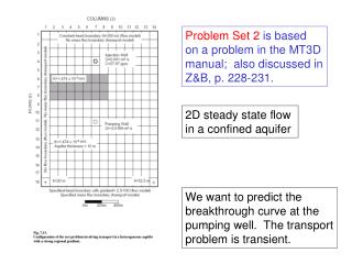
Problem Set 2 is based on a problem in the MT3D manual; also discussed in Z&B, p. 228-231. 2D steady state flow in a confined aquifer. We want to predict the breakthrough curve at the pumping well. The transport problem is transient. Zone of low hydraulic conductivity.

E N D
Problem Set 2 is based on a problem in the MT3D manual; also discussed in Z&B, p. 228-231. 2D steady state flow in a confined aquifer We want to predict the breakthrough curve at the pumping well. The transport problem is transient.
Zone of low hydraulic conductivity Peclet numbers = 5 and 25
GWV screen Note: the heterogeneity is not present in the first column
Units in MT3D – see p. 6-8 in the manual Concentration units do not have to be consistent with the units used for other parameters. It is permissible, for example, to use “ft” for the system parameters and mg/l for concentration. However, in that case the units calculated in the mass balance will have inconsistent units and the mass balance numbers will need to be manually corrected. Recommended: use ppm= mg/l gm/m3 That is, use meters; mass is reported in grams. Mass = c Q t
Cs = 0 Cs = 57.87 ppm
NOTE. These results were produced using an old version of MT3DMS. Please run again with the latest version of the code.
MT3DMS Solution Options PS#2 1 3 4 2
Central Difference Solution Time step multiplier = 1 41 time steps Time step multiplier = 1.2 13 time steps
Courant number See information on solution methodologies under the MT3DMS tab on the course homepage for more about these parameters.
Boundary Conditions ---for flow problem ---for transport problem
Head solution-- Flow problem is steady state
Need to designate these boundary cells as inactive concentration cells. Use zone 10 in the diffusions properties menu of Groundwater Vistas.
Cells in first row are in zone 10 in the diffusion properties menu This is necessary to prevent loss of mass through the boundary by diffusion.
Mass Balance Considerations in MT3DMS Sources of mass balance information: *.out file *.mas file mass balance summary in GW Vistas See supplemental information for PS#2 posted on the course homepage for more information on mass balance options.
Water Flow: IN= through upper boundary; injection well OUT= pumping well; lower boundary wells IN - OUT = S where S = 0 at steady state conditions Mass Flux: IN= through injection well; changes in storage OUT= pumping well; lower boundary; changes in storage Mass Balance states that: Mass IN = Mass OUT where changes in mass storage are considered either as contributions to mass IN or to mass OUT.
From the *.out file (TVD solution)
Mass Storage: Water Consider a cell in the model IN - OUT = S where change in storage is S = S(t2) – S(t1) If IN > OUT, the water level rises and there is an increase in mass of water in the cell. IN = OUT + S, where S is positive. Note that S is on the OUT side of the equation. If OUT > IN IN – S = OUT, where S is negative S is on the IN side of the equation.
From the *.out file (TVD solution) S S = c (x y z )
Mass Storage: Solute IN - OUT = S where change in storage is S = S(t2) – S(t1) If IN > OUT, concentration in cell increases and there is an increase in solute mass in the cell. IN = OUT + S, where S is positive. Note that S is on the OUT side of the equation. There is an apparent “sink” inside the cell. If OUT > IN, the concentration in cell decreases and there is a decrease in solute mass in the cell. IN – S = OUT, where S is negative and S is on the IN side of the equation. There is an apparent “source” inside the cell.
From the *.out file (TVD solution) S IN – OUT = 0 (INsource+SIN) - (OUTsource + SOUT)= 0 SIN - SOUT = Storage
HMOC *.mas file q’s =
q’s = General form of the ADE: Expands to 9 terms Expands to 3 terms Where does the extra term come from? (See eqn. 3.48 in Z&B)
Isotherms Assume local chemical equilibrium (LEA):
MOC methods typically report high mass balance errors, especially at early times.
S IN – OUT = 0 (INsource+SIN) - (OUTsource + SOUT)= 0 SIN - SOUT = Storage From the *.out file (TVD solution)
From the *.out file (TVD solution)
Last t = 0.0089422 yr Mass Flux = (mass at t2 - mass at t1) / t