The Fundamental Theorem of Calculus
Learn how the Fundamental Theorem connects differential and integral calculus, and how it relates to functions defined by equations. Explore examples and illustrations to grasp the essence of this fundamental concept in mathematics.


The Fundamental Theorem of Calculus
E N D
Presentation Transcript
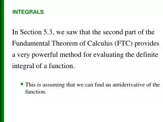
The Fundamental Theorem of Calculus • The Fundamental Theorem of Calculus is appropriately named because it establishes a connection between the two branches of calculus: differential calculus and integral calculus. • It gives the precise inverse relationship between the • derivative and the integral.
The Fundamental Theorem of Calculus • The first part of the Fundamental Theorem deals with functions defined by an equation of the form • where f is a continuous function on [a, b] and x varies between a and b. Observe that g depends only on x, which appears as the variable upper limit in the integral. If x is a fixed number, then the integral is a definite number. • If we then let x vary, the number also varies and defines a function of x denoted by g(x).
The Fundamental Theorem of Calculus • If f happens to be a positive function, then g(x) can be interpreted as the area under the graph of f from a to x, where x can vary from a to b. (Think of g as the “area so far” function; see Figure 1.) Figure 1
Example 1 – A Function Defined as an Integral • If f is the function whose graph is shown in Figure 2 and find the values of g(0), g(1), g(2), g(3), g(4), • and g(5). Then sketch a rough graph of g. Figure 2
Example 1 – Solution • First we notice that . • From Figure 3(i) we see that g(1) is the area of a triangle: • To find g(2) we again refer to Figure 3(ii) and add to g(1) the area of a rectangle: = (1 2) = 1 Figure 3(i) = 1 + (1 2) = 3 Figure 3(ii)
Example 1 – Solution cont’d • We estimate that the area under f from 2 to 3 is about 1.3, so • For t 3, f(t) is negative and so we start subtracting areas: 3 + 1.3 = 4.3 Figure 3(iii) 4.3 + (–1.3) = 3.0 Figure 3(iv)
Example 1 – Solution cont’d • We use these values to sketch the graph of g in Figure 4. • Notice that, because f(t) is positive for t 3, we keep adding area for t 3 and so g is increasing up to x = 3, where it attains a maximum value. For x 3, g decreases because f(t) is negative. 3 + (–1.3) = 1.7 Figure 3(v) Figure 4
The Fundamental Theorem of Calculus • For the function, where a = 1 and f(t) = t2, notice that g(x) = x2, that is, g = f. In other words, if g is defined as the integral of f by Equation 1, then g turns out to be an antiderivative of f, at least in this case. • And if we sketch the derivative of the function g shown in Figure 4 by estimating slopes of tangents, we get a graph like that of f in Figure 2. So we suspect that g = f in Example 1 too. Figure 2
The Fundamental Theorem of Calculus • To see why this might be generally true we consider any continuous function f with f(x) 0. Then can be interpreted as the area under the graph of f from a to x, as in Figure 1. • In order to compute g(x) from the definition of a derivative we first observe that, for h 0, g(x + h) – g(x) is obtained by subtracting areas, so it is the area under the graph of f from x to x + h (the blue area in Figure 5). Figure 1 Figure 5
The Fundamental Theorem of Calculus • For small h you can see from the figure that this area is approximately equal to the area of the rectangle with height f(x) and width h: • g(x + h) – g(x) hf(x) • so • Intuitively, we therefore expect that
The Fundamental Theorem of Calculus • The fact that this is true, even when f is not necessarily positive, is the first part of the Fundamental Theorem of Calculus. • Using Leibniz notation for derivatives, we can write this theorem as • when f is continuous.
The Fundamental Theorem of Calculus • Roughly speaking, this equation says that if we first integrate f and then differentiate the result, we get back to the original function f. • It is easy to prove the Fundamental Theorem if we make the assumption that f possesses an antiderivative F. Then, by the Evaluation Theorem, • for any x between a and b. Therefore • as required.
Example 3 – Differentiating an Integral • Find the derivative of the function • Solution: • Since is continuous, Part 1 of the • Fundamental Theorem of Calculus gives
Example 4 – A Function from Physics • Although a formula of the form may seem like a strange way of defining a function, books on physics, chemistry, and statistics are full of such functions. For instance, the Fresnel function • is named after the French physicist Augustin Fresnel (1788–1827), who is famous for his works in optics. • This function first appeared in Fresnel’s theory of the diffraction of light waves, but more recently it has been applied to the design of highways.
Example 4 – A Function from Physics cont’d • Part 1 of the Fundamental Theorem tells us how to differentiate the Fresnel function: • This means that we can apply all the methods of differential calculus to analyze S. • Figure 6 shows the graphs of f(x) = sin(x2/2) and the Fresnel function Figure 6
Example 4 – A Function from Physics cont’d • A computer was used to graph S by computing the value of this integral for many values of x. • It does indeed look as if S(x) is the area under the graph of f from 0 to x [until x 1.4when S(x) becomes a difference of areas]. Figure 7 shows a larger part of the graph of S. Figure 7
Example 4 – A Function from Physics cont’d • If we now start with the graph of S in Figure 6 and think about what its derivative should look like, it seems reasonable that S(x) = f(x). [For instance, S is increasingwhen f(x) 0 and decreasing when f(x) 0.] So this gives a visual confirmation of Part 1 of the Fundamental Theorem of Calculus. Figure 6
Differentiation and Integration as Inverse Processes • We now bring together the two parts of the Fundamental Theorem. • We noted that Part 1 can be rewritten as • which says that if f is integrated and then the result is differentiated, we arrive back at the original function f.
Differentiation and Integration as Inverse Processes • We have reformulated Part 2 as the Net Change Theorem: • This version says that if we take a function F, first differentiate it, and then integrate the result, we arrive back at the original function F, but in the form F(b) – F(a). • Taken together, the two parts of the Fundamental Theorem of Calculus say that differentiation and integration are inverse processes. Each undoes what the other does.