OOO Pipelines - III
OOO Pipelines - III. Smruti R. Sarangi Computer Science and Engineering, IIT Delhi. Contents. OOO Processor with an Architectural Register File Aggressive Speculation and Replay Uses of Aggressive Speculation. Let us now look at a different kind of OOO processor.

OOO Pipelines - III
E N D
Presentation Transcript
OOO Pipelines - III Smruti R. Sarangi Computer Science and Engineering, IIT Delhi
Contents • OOO Processor with an Architectural Register File • Aggressive Speculation and Replay • Uses of Aggressive Speculation
Let us now look at a different kind of OOO processor • Instead of having a physical register file, let us have an architectural register file(ARF) • A 16-entry architectural register file that contains the committed architectural state. Commit Time Rest remains the same Committed State ARF IW Renaming Decode Register Write ROB Temporary State Write back temp. results
Changes to renaming • Entry in the RAT (register address translation) table Entry in the RAT table ROB/RF bit ROB id • ROB/RF bit 1 (value in the ROB), 0 (value in the RF) • Use the ROB if the ROB/RF bit indicates that the value is in the ROB • Entry in the ROB: (ready bit indicates if the value is in the ROB (1) or being generated in the pipeline (0)) Entry in the ROB value dest Instruction ready dest
Changes to Dispatch and Wakeup • Each entry in the IW now stores the values of the operands • Reason: We will not be accessing the RF again • What is the tag in this case? • It is not the id of the physical register. • It is the id of the ROB entry. • What else? • Along with the tag we need to broadcast the value of the operand also if we will not get the value from the bypass network • This will make the circuit slower
Changes to Wakeup, Bypass, Reg. Write and Commit • We can follow the same speculative wakeup strategy and broadcast a tag (in this case, id of ROB entry) immediately after an instruction is selected • Instructions directly proceed from the select unit to the execution units • All tags are ROB ids. • After execution write the result to the ROB entry • Commit is simple. We have always the architectural state in the ARF. • We just need to flush the ROB.
PRF based design vs ARF based design • + points in the PRF based design • A value resides in only a single location (PRF). Multiple copies of values are never maintained. In a 64-bit machine, a value is 64 bits wide. • Each entry in the IW is smaller (values are not saved). • The broadcast is also narrower • Restoring state is complicated • + points in the ARF based design • Recovery from misspeculationis easy • We do not need a free list • Values are maintained at multiple places (ARF, ROB, IW)
Contents • OOO Processor with an Architectural Register File • Aggressive Speculation and Replay • Uses of Aggressive Speculation
Aggressive Speculation • Branch prediction is one form of speculation • If we detect that a branch has been mispredicted • Solution: flush the pipeline • This is not the only form of speculation • Another very common type: load latency speculation • Assume that a load will hit in the cache • Speculatively wakeup instructions • Later on if this is not the case: DO SOMETHING
Replay • Flushing the pipeline for every misspeculation is not a wise thing • Instead, flush a part of the pipeline (or only those instructions that have gotten a wrong value) • Replay those instructions once again (after let’s say the load completes its execution) • When the instructions are being replayed, they are guaranteed to use the correct value of the load
Two methods of replaying • Method 1: Keep instructions that have been issued in the issue queue (see reference) verification status IW Pipeline Stages Verify remove from issue queue if verified
Two methods of replaying - II • Move the instructions to a dedicated replay queue after issue • Once an instruction is verified remove it from the replay queue verification status Verify Pipeline Stages IW Replay queue remove from replay queue if verified remove from the issue queue
Non-Selective Replay • Trivial Solution: Flush the pipeline between the schedule and execute stages • Smarter Solution • It is not necessary to flush all the instructions between the schedule and execute stages • Try to reduce the set of instructions • Define a window of vulnerability (WV) for n cycles after a load is selected. A load should complete within n cycles if it hits in the d-cache and does not wait in the LSQ • However, if the load takes more than n cycles, we need to do a replay • Algorithm: Kill all
Instruction Window Entry Broadcast bus • When an instruction wakes up, we set the timer to n • Every cycle it decrements (count down timer) • Once it becomes 0, we can conclude that this instruction will not be squashed Kill wire tag ready bit Timer
More about Non-Selective Replay • We attach the expected latency with each instruction packet as it flows down the pipeline • Wherever there is an additional delay (such as cache miss) • Time for a replay • Set the kill wire • Each instruction window entry that has a non-zero count, resets its ready flag • We now have a set of instructions that will be replayed • For some such instructions tags will be broadcast • Not for all (see the next slide)
Example ld r1, 8[r4] add r2, r1, r1 sub r4, r3, r2 xor r5, r6, r7 • Assume that the loadinstruction misses in the L1 cache • The add, sub, and xor instructions will need to be squashed, and replayed • For the add and sub instructions tag will be broadcast • What about the xor instruction? • We need to broadcast additional tags
Delayed Selective Replay • Let us now propose an idea to replay only those instructions that are in the transitive-closure of the misspeculatedload • Let us extend the non-selective replay scheme • At the time of asserting the kill signal, plant a poison bit in the destination register of the load • Propagate the bit along the bypass paths and through the register file • If an instruction reads any operand whose poison bit is set, then the instruction’s poison bit is also set. • When an instruction finishes execution
Delayed Selective Replay - II • When an instruction finishes execution • Check if its poison bit is set. • If yes, squash it • If no, re-enable the instruction and broadcast a message to mark the instruction ready • Issues with this scheme • It is effective, but, assumes that we know the value: n • This might not be possible all the time • Dependent instructions get the verification status by timing out. This creates some false dependences also
Token Based Selective Replay • Let us use a pattern found in most programs: • Most of the misses in the data cache are accounted for by a relatively small number of instructions • 90/10 thumb rule 90% of the misses are accounted for by 10% of instructions • Predictor Given a PC, predict if it will lead to a d-cache miss • Use a predictor similar to a branch predictor at the fetch stage Prediction Table PC Output
After Predicting d-cache Misses • Instructions that are predicted to miss, will have a non-deterministic execution time (most likely) and lead to replays (set S1) • Other instructions will not lead to replays (most likely) (set S2) • Let us consider an instruction in set S1 • At decode time, let the instruction collect a free token • Save the id of the token in the instruction packet • Example: assume the instruction: ld r1, 4[r4] is predicted to miss • Save the id of the token in the instruction packet of this instruction • Say that the instruction gets token #5 • This instruction is the token head for token #5 • Let us propagate this information to all the instructions dependent on the load • If this load fails, all the dependent instructions fail as well
Structure of the Rename Table rename table phy. reg • If an instruction is a token head, we save the id of the token that it owns • Assume we have a maximum of N tokens. tokenVec is a N-bit vector • For the token head instruction, if it owns the ith token, set the ith bit to true in tokenVec r1 id of token tokenVec
While reading the rename table ... add r1, r2, r3 • Read the tokenVecsof the sourceoperands • Merge the tokenVecs of the source operands • Save the merged tokenVecfor the destination register (in the rename table)
After execution • After the token head instruction completes execution, see if it took additional cycles • If YES, broadcast the token id to signal a replay (Case 1) • If NO, broadcast the token id to all the instructions. They can turn the corresponding bit off. (Case 2) Case 2 Case 1 Replay
Instructions in S2 • Assume an instruction that was not predicted to miss actually misses • No token is attached to it • Solution: • Squash all instructions after this instruction from the IW • Re-insert them from the ROB • Expensive Operation • The replay mechanism is cheaper than a full scale pipeline flush
Contents • OOO Processor with an Architectural Register File • Aggressive Speculation and Replay • Uses of Aggressive Speculation
What can we predict? • Data obtained from the L1 cache • Dependences between load-store instructions • Load instructions that will most likely read data from the L1 cache and have a cache hit • ALU results
Why can we predict? (Lipasti and Shen, ’96) • Data redundancy • Bit masking operations • Trivial operands and constants • Results of error checking • Code for virtual functions • Glue code • Register spill code
How to Predict? Confidence Table (uses sat. counters) Predictor Table PC PC Confidence Prediction • First, use the confidence table to find out if it makes sense to predict • Simultaneously, make a prediction using a predictor table (value, memory dependence, ALU result) • Predictor table can contain 1 value, or the last kvalues • Make a prediction, and use it if it has high confidence • Update both the tables when the results are available • If needed recover with a replay/flush mechanism