Download
1 / 18
180 likes | 272 Vues
Explore the dynamics of chaos theory in business cycles, derived from natural sciences and applicable to distribution battles. Learn about bifurcations, fixed points, and economic applications in the Goodwin/Pohjola model. Discover strengths, weaknesses, and critical analysis.

E N D
6. Chaos-Theory and the Business Cycle • Endogenousand real businesscycles • Derivedfromnaturalsciences • Flourished in 1980s and 1990s • Meanwhile out offashionagain (tootechnical, lackingpolicyreceipts) • But interestinginsights in dynamics, applicabletodistribution-battle 1 U van Suntum, Vorlesung KuB 1
Chaos-theory: An example*) x t+1 = r xt(1 – xt) Xmax = 0,25 r x t+1 xt 0 0,5 1,0 *) cf. Ian Stewart, Spielt Gott Roulette? Chaos in der Mathematik, Basel u.a. 1990, S. 163 ff.; Heubes, Konjunktur u. Wachstum, a.a.O., S. 108 KuKuB 7 2 KuB 7 U van Suntum, Vorlesung KuB 2
Derivation of maximum: x t+1 = r xt(1 – xt) Xmax = 0,25 r x t+1 0,5 xt 3 KuB 7 U van Suntum, Vorlesung KuB 3
Derivation of fixed point (equlibrium): x t+1 = r xt (1 – xt) 45o x t+1 = xt Xmax = 0,25 r x t+1 „fixed point“ 0,5 xt Existenceofequilibriumis not sufficienttoguaranteeitsfeasibilityandstability! 4 KuB 7 U van Suntum, Vorlesung KuB 4
x t+1 = r xt (1 – xt) Y t+1 = aYt (1 – Yt) • with 0 < r < 3 => convergence to fixed point • with 3 < r < 3,58 => fluctuations (bifurcations) • with 3,58 < r < 4 => chaos with occasional periodicity • with r > 4 => exploding Chaosgleichungbeispiel.xls Fixed point (stable if absolute slope of curve < 1) Xmax = 0,25 r x t+1 45o Points which are feasible in principle xt Startwert 5 KuB 7 U van Suntum, Vorlesung KuB 5
a) convergence (0 < r < 3); here: r = 2,8 => fixed point = 0,6428 fixed point: x = 0,6428 start: x = 0,4 temporal behavior of x 6 KuB 7 U van Suntum, Vorlesung KuB 6
b) bifurcations (3 < r < 3,58); here: r = 3,2 => fixed point = 0,6875 points of bifurcation:*) x = 0, 7995 und x = 0,5130 start: x = 0,4 *) numericallyderived by Excel-Solver: conditions: x t+1 = x t+3 and x t+2 = x t+4 temporal behavior of x 7 KuB 7 U van Suntum, Vorlesung KuB 7
c) chaos (3,58 < r < 4); here: r = 3,8 => fixed point = 0,7368 start: x = 0,4 temporal behavior of x 8 KuB 7 U van Suntum, Vorlesung KuB 8
d) explosion ( r > 4); here: r = 4,2 start: x = 0,4 temporal behavior of x 9 KuB 7 U van Suntum, Vorlesung KuB 9
Economic application: Goodwin/Pohjola-model (1967/1981) (cf. Heubes, Konjunktur und Wachstum) • wages w (and wage share u = W/Y) rise in Y • grwoth rate gY declines in wage share u (1 – u) g u u g (1 – u) 10 KuB 7 U van Suntum, Vorlesung KuB 10
Application: Business Cycle Model of Goodwin/Pohjola (1967/1981) • Assumptions: • Leontief production function=> g denotes growth rate of Y, K and N • Classical saving function: amount G is saved, amount W consumed • Additional simplifications here: no technical progress, size of labor force fixed • Wages increase in employment and labor productivity Variables: I = investment, K = capital stock, N= labor, k = capital coefficient K/Y, w = wage rate , d = wage adjustment parameter, N* = equilibrium employment (fixed point of chaos model) 11 KuB 7 U van Suntum, Vorlesung KuB 11
Formal Derivation of Goodwin/Pohjola-Model chaos with k < 0,39 KuB 7 U van Suntum, Vorlesung KuB 12 12
Chaosgleichungbeispiel.xls • Explanation: • investment proportional to profit share (1-u) because all profits are saved (eq.1) • employment proportional to total income because of Leontief PF (eq. 2) • high employment and high productivity increase wage rate (eq. 3) • model culminates in a single difference equation (eq. 6, 7). • thus with given starting point N and constant N* employment is determined at any t • empirical estimation by autoregressive methods (using only Nt, Nt-1 etc.) KuKuB 7 13 KuB 7 U van Suntum, Vorlesung KuB 13
Grafical exposition with k < 0,39 (here: k = 0,38) employment N(t) KuKuB 7 14 KuB 7 U van Suntum, Vorlesung KuB 14
bifurcation with k > 0,4 (here: k = 0,6) Damped fluctuations with k >> 0,4 (here: k = 0,6) employment N(t) employment N(t) Summary: anything goes… 15 KuB 7 U van Suntum, Vorlesung KuB 15
Strengths: Shows dynamics of business cycle Easily transformable into econometrics Can explain erratic fluctuations Weaknesses: technical, relatively little economic content Poor policy relevance Very simple economic model Critique of Chaos-Theory 16 KuB 7 U van Suntum, Vorlesung KuB 16
How do mathematicans and economists define chaos? What is the fixed point of a dynamic model? What are bifurcations? Where do the dynamics in the Goodwin/Pohjola model come from? How does the wage share behave over the business cycle? Lerning goals/Questions 17 KuB 7 U van Suntum, Vorlesung KuB 17
Exercise: Assume the following difference equation for total demand in the business cycle: • Letparameter a be 4.20 • Whatisthemaximumpossiblevalueof Y? • Whatisthefixedpointofthe model? KuKuB 7 18 KuB 7