Download
1 / 61
610 likes | 724 Vues
Delve into the intricate world of climate dynamics with a focus on time scales, sensitivity, and the components of global warming. From shifting latitudes to hydrological cycles, explore the key elements shaping our climate. Discover the importance of ocean heat uptake efficacy in transient climate change and the uncertainties surrounding climate sensitivity assessments.

E N D
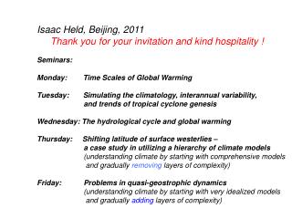
Isaac Held, Beijing, 2011 Thank you for your invitation and kind hospitality ! Seminars: Monday: Time Scales of Global Warming Tuesday: Simulating the climatology, interannual variability, and trends of tropical cyclone genesis Wednesday: The hydrological cycle and global warming Thursday: Shifting latitude of surface westerlies – a case study in utilizing a hierarchy of climate models (understanding climate by starting with comprehensive models and gradually removing layers of complexity) Friday: Problems in quasi-geostrophic dynamics (understanding climate by starting with very idealized models and gradually adding layers of complexity)
Time scales of climate responses, climate sensitivity, and the recalcitrant component of global warming Isaac Held Beijing, 2011 Importance of Ocean Heat Uptake Efficacy to Transient Climate Change Winton, Takahashi, Held, J. Clim, 2010 Probing the fast and slow components of global warming by returning abruptly to pre-industrial forcing Held, Winton, Takahashi, Delworth, Zeng, Vallis, J. Clim 2010
Uncertainty in climate sensitivity has not been reduced appreciably in past 30 years 2 well-known assessments reach similar conclusions : “Charney report” (1979) IPCC/AR4 (2006) Equilibrium global mean surface temperature warming due to doubling of CO2 is most probably in the range 1.5-4.5 K
Assorted estimates of equilibrium sensitivity Knutti+Hegerl, 2008 23
Time scales of climate response Ultra-fast Fast Slow Ultra-slow Months (Atmosphere) a few years (mixed layer) Multiple centuries (deep ocean)
Equilibrium climate sensitivity: Double the CO2 and wait for the system to equilibrate Transient climate response: Increase CO2 1%/yr and examine climate at the time of doubling Typical setup – increase till doubling – then hold constant CO2 forcing T response W/m2 t Heat uptake by deep ocean After CO2 stabilized, warming of near surface can be thought of as due to reduction in heat uptake 11
CMIP3/AR4 models 2.5 2 Transient response 1.5 1 2 3 4 5 Equilibrium sensitivity Not well correlated across models – equilibrium response brings into play feedbacks/dynamics (especially in subpolar oceans) that are suppressed in transient response 19
Histogram of TCR/TEQ for AR4 models Increase CO2 by 1%/yr ; global mean warming at the time of doubling = Transient Climate Response (TCR)
Response of global mean temperature in GFDL’s CM2.1 to instantaneous doubling of CO2 Equilibrium sensitivity 3.4K Transient response 1.5K Slow response evident only after 80 yrs Fast response 20
forcing Mixed layer Heat capacity Heat exchange between mixed layer and deep ocean Deep ocean heat capacity in equilibrium
Forcing varies on time scales longer than and time scales shorter than “Intermediate regime”
Forcing computed from differencing TOA fluxes in two runs of a model (B-A) B = fixed SSTs with varying forcing agents; A fixed SSTs and fixed forcing agents total OLR SW down 51 SW up
Temperature change averaged over 5 realizations of coupled model 52
Fit with 53
Forcing (with no damping) fits the trend well, if you use transient climate sensitivity, which takes into account magnitude/efficacy of heat uptake Forcing with no damping 54
GFDL’s CM2.1 with well-mixed greenhouse gases only Global mean temperature change Observations (GISS) 46
GFDL’s CM2.1 with well-mixed greenhouse gases only Global mean temperature change Observations (GISS) “It is likely that increases in greenhouse gas concentrations alone would have caused more warming than observed because volcanic and anthropogenic aerosols have offset some warming that would otherwise have taken place.” (AR4 WG1 SPM). 46
Return instantaneously to pre-industrial forcing ( F = 0) the “Recalcitrant” warming
Relaxation to recalcitrant warming 5 years 3 years
Normalized to unity over the globe Fast Slow “Recalcitrant”
Sea level response due to thermal expansion Control drift Sea level response mostly recalcitrant
The simplest linear model If correct, evolution should be along the diagonal N/F T/TEQ 15
Suppose you have two forcing agents C02 and B (something else) leading to radiative forcing FC02 and FB . But suppose the global mean temperature responses TC02 and TB are not proportional to the the radiative forcing Following Hansen, define efficacy eB (using CO2 as a standard)
Efficacy can orten be understood in terms of the spatial structure of the response , Coupling of surface with troposphere is weaker in high latitudes => harder to radiate away a perturbation => Radiative restoring strength is weaker for responses that are larger in higher latitudes => Forcings with stronger high latitude responses have larger efficacy
Forcings with stronger high latitude responses have larger efficacy Think of heat uptake as a forcing – ie replace F = bT + H or bT = F + H with bT = F + eH H with eH > 1 Equivalently, T = TF + TH = F/b - H/bH With bH = b/eH
Heat uptake = gT ; g = efficiency of heat uptake Cooling due to heat uptake = egT ; e = efficacy of heat uptake Efficiency CM 2.1 CM 2.0 Efficacy
Assorted estimates of equilibrium sensitivity Knutti+Hegerl, 2008 23
(GFDL CM2.1 -- Includes estimates of volcanic and anthropogenic aerosols, as well as estimates of variations in solar irradiance) Models can produce very good fits by including aerosol effects, but models with stronger aerosol forcing and higher climate sensitivity are also viable (and vice-versa) 45
Observational constraints • 20th century warming • 1000yr record • Ice ages – LGM • Deep time • Volcanoes • Solar cycle • Internal Fluctuations • Seasonal cycle etc 36
Observed total solar irradiance variations in 11yr solar cycle (~ 0.2% peak-to-peak) 42
Camp and Tung, 2007 => 0.2K peak to peak (other studies yield ~0.1K) Seems to imply large sensitivity 4 yr damping time Only gives 0.05 peak to peak 1.8K (transient) sensitivity 43
Global mean cooling due to Pinatubo volcanic eruption Observations with El Nino removed Range of ~10 Model Simulations GFDL CM2.1 Courtesy of G Stenchikov 40 Relaxation time after abrupt cooling contains information on climate sensitivity
Low sensitivity model Pinatubo simulation High sensitivity model Yokohata, et al, 2005 41
Response to pulse of forcing (volcano), F(t): 2-box model:
Near surface air temperature response (20 member ensemble) Courtesy of Stenchikov, et al
Integrated forcing and response Wm-2yr Response with exponential fit TOA flux Forcing
CM2.1 Pinatubo summary -- fast response --
Radiative restoring (W/m2)yr 2.8 Forcing (W/m2)yr 5.0 Heat uptake (W/m2)yr 2.2 CM2.1 Pinatubo summary -- fast response --
Pinatubo => b ~ 1.0 (W/m2)/K g ~ 0.8 (W/m2)/K 1%/yr CO2 increase => b ~ 1.7 (W/m2)/K g ~ 0.7 (W/m2)/K
Can we use interannual variability to determine the strength of the radiative restoring? Model results (CM2.1) raise some roadblocks
Longwave regression across ensemble (collaboration with K. Swanson) All-forcing 20th century bLW Wm-2K-1 year 61 Following an idea of K. Swanson, take a set of realizations of the 20th century from one model, and correlate global mean TOA with surface temperature across the ensemble
Longwave regression across ensemble, collaboration with K. Swanson All-forcing 20th century A1B scenario bLW Wm-2K-1 62