Chapter 2: Dynamic Models
Chapter 2: Dynamic Models. Part B: Differential Equations in State-Variable Form. Material covered in the P RESENT L ECTURE is shown in yellow. I. DYNAMIC MODELING Deriving a dynamic model for mechanical , electrical, electromechanical, fluid- & heat-flow systems

Chapter 2: Dynamic Models
E N D
Presentation Transcript
Chapter 2: Dynamic Models Part B: Differential Equations in State-Variable Form
Material covered in the PRESENT LECTURE is shown in yellow I. DYNAMIC MODELING • Deriving a dynamic model formechanical, electrical, electromechanical, fluid- & heat-flow systems • Linearization the dynamic model if necessary II. DESIGN OF A CONTROLLER: Several design methods exist • Classical control or Root Locus Design: Define the transfer function; Apply root locus, loop shaping,… • Modern control or State-Space Design: Convert ODE to state equation; Apply Pole Placement, Robust control, … • Nonlinear control: Apply Lyapunov’s stability criterion
Motivations for Deriving the Dynamic Model in STATE-VARIABLE FORM • Be able to apply the State-Space design method (more on this later) • Enhances our ability to apply the computational efficiency of analysis tools such as MATLAB, since the state-variable form is one of the methods used for specifying differential equations in computer-aided control systems design software packages.
Foundation • Use of Newton’s law typically leads to SECOND-order differential equations, that is equations that contain a second derivative of the system variables such as: • These differential equations also can be expressed as a set of simultaneous FIRST-order differential equations.
Foundation - Example • Consider a system composed of a single mass (m), attached to a spring (k) and a damper (b), submitted to an external force (u) and characterized by the following dynamic model: • (1) can be rewritten as follows: (1) (1a) by defining v as: (1b) (1)(1a) & (1b)
State-Variables: Recall Example • x is the variable that describe any arbitrary position of the system (also called system variable) • are the state-variables of the system. • Since , the state-variables can be defined as
State-Variable Form Deriving differential equations in state-variable form consists of writing them as a vector equation as follows: whereis the output and u is the input
is called state of the system. X is the state vector.It contains n elements for an nth-order system, which are the n state-variables of the system. Definitions You can forget that Important • The constant J is called direct transmission term
Deriving the State-Variable Form requires to specifyF, G, H, J for a given X and u
Ex 1: Recall the Satellite Altitude Control Example Assumptions: • is the angular velocity • The desired system output isθ Q:Dynamic model in state-variable form?
Strategy (recommended but not required) • Derive the dynamic model. • Identify the input control variable, denoted by u. • Identify the output variable, denoted by y. • Define a state vector, X , having for elements the system variables and their first derivative. • Determine • Determine F and G, in manner that • Determine H and J, in manner that
Ex 1: Dynamic Model • Applying Newton’s law for 1-D rotational motion leads to: => (1)
Given: The control input, denoted by u, is given by: The output, denoted by y, is the displacement angle: y = θ Assumption: The state vector, denoted by X, is defined as: Known: The dynamic model (1) Required: Rewrite (1) as: Example 1 (cont’d)
Example 1 (cont’d) • By definition: . As a result, • Expressing the dynamic model: as a function of ωand u (with) yields: (1)
Available equations: From the dynamic model: The output y is defined as: y = θ The input u is given by: Equivalent form of available eq: where and Therefore: Example 1 (cont’d)
Example 1: Dynamic Model in State-Variable Form By defining X and u as: The state-variable form is given by: input state-variables
Ex 1½: Recall the Satellite Altitude Control Example Assumptions: • is the angular velocity • The system output isω Q:Dynamic model in state-variable form?
Example 1½: Dynamic Model in State-Variable Form By defining X and u as: The state-variable form is given by: Only change
Analysis in Control Systems • Step 1: Derive a dynamic model • Step 2: Specifying the dynamic model to software by writing it in STATE-VARIABLE form in terms of its TRANSFER FUNCTION(see chapter 3) either or
Example 2: Cruise Control Step Response • Q1: Rewrite the equation of motion in state-variable formwhere the output is the car velocity v? • Q2: Use MATLAB to find the step response of the velocity of the car ? • Assume that the input jumps from being u(t) = 0 N at time • t = 0 sec to a constant u(t) = 500 N thereafter.
Reminder: Strategy • Derive the dynamic model. • Identify the input control variable, denoted by u. • Identify the output variable, denoted by y. • Define a state vector, X , having for elements the system variables and their first derivative. • Determine • Determine F and G, in manner that • Determine H and J, in manner that
Ex 2, Q1:Dynamic Model • Applying Newton’s law for translational motion yields: (2) =>
Given: The input ( = external force applied to the system) is denoted by u The output, denoted by y, is the car’s velocity: y = v Assumption: The state-vector is defined as: Known: The dynamic model (2) Required: Rewrite (2) as: Example 2, Question 1 (cont’d)
Example 1 (cont’d) • By definition: . As a result, • Expressing the dynamic model: as a function of v and u leads to: (2)
Available equations: From the dynamic model: The output y is defined as: y = v The input is the step function u Equivalent form of available eq: where Therefore: Ex 2, Q1 (cont’d)
Example 2, Question 1: Dynamic Model in State-Variable Form By defining X as: The state-variable form is given by:
Example 2, Question2: Step Response using MATLAB? Assumptions:m = 1000 kg and b= 50 N.sec/m.
Ex 2, Q2: Step Response with MATLAB? • The step function in MATLAB calculates the time response of a linear system to a unit step input. • In the problem at hand, the input u is a step function of amplitude 500 N: u = 500* unity step function. • Because the system is linear ( ): G * u = (500 * G) * unitystep function G * Step 0 to 500 N 500*G * Step 0 to 1 N
F = [0 1;0 -0.05]; G = [0;0.001]; H = [0 1]; J = 0; sys = ss(F, 500*G, H, J); t = 0:0.2:100; y = step(sys,t); plot (t,y) % defines state variable matrices % defines system by its state- space matrices % setup time vector ( dt = 0.2 sec) % computes the response to a unity step response % plots output (i.e., step response) MATLAB Statements
Response of the car velocity to a step input u of amplitude 500 N
Example 3: Flexible Disk-Drive Q:Find the state-variable form of the differential equations describing the dynamics of the systemif the output is the rotation angle2? Note: Define the state vector to be
Example 3: Dynamic Model • Newton’s law for 1-D rotational motion yields to:
Example 3: Dynamic Model in State-Variable Form By defining X and u as: The state-variable form is given by: