Download
1 / 29
290 likes | 391 Vues
Explore the modeling and visualization of cometary phenomena like the evaporation process using computer-generated images. Learn the principles and techniques through a Java Applet simulation.

E N D
Course Name: Programming Mini-project 2 • Theme: Computer generated pictures of comets http://cis.k.hosei.ac.jp/~vsavchen/MiniPr_2/
Introduction • One of the challenging problems of computer graphics (CG) and computer arts is the visualization of different natural phenomena and simulated flow data. • Examples are clouds, space phenomena such as evaporation process of comet nucleus, mirages, rainbows, and other atmospheric effects. • Visualization of simulated data can be useful in different application areas to display behavior of studied phenomena or to improve CG images with more correct scientific factors.
Introduction • An example of evaporation process of comet nucleus • One process which transfers water from the ground back to the atmosphere is evaporation. Evaporation is when water passes from a liquid phase to a gas phase. • The head of Comet Halley, May 1910. Photographed at Helwan Observatory, Egypt
Introduction • Characteristics of a Comet • Structure • Nucleus • Coma • Dust tail • Plasma tail • Evaporation process • When a comet approaches within a few AU of the Sun, the surface of the nucleus begins to warm, and volatiles evaporate. The evaporated molecules boil off and carry small solid particles with them, forming the comet's coma of gas and dust. • Begins inside of Mar’s orbit Generating coma and two tails
Introduction • Modeling and Visualization of a Cometary Coma • To get the optical picture of a cometary coma, we can use simple particle-based simulation, however, based on the main premises of the Whipple’s theory. • According to this theory the cometary nucleus is an icy conglomerate of dust and meteor material. • The icy particles evaporate on the surface exposed to the sun and carry off the dust particles accelerated by the solar radiation. • For more references, see, Whipple F. L. (1950) A comet model I. The acceleration of Comet Encke. Astrophys. J., 111, 375–394. Bschorr, O.; Jochim, E.F.; Freund, J. (1979) Computer-GeneratedPictures of Comets'. :l. IAF-Congress, Amsterdam, 30 Sep-5 Oct 1974
Introduction • The optical picture of the coma and tail is visualized by a Java Applet.
Introduction. Newtonian particle systems • A particle is described by its mass, m, and its trajectory, r(t), as illustrated in Figure • Newtonian particles are the most common and are governed by Newton’s second low • F = md2r(t)/dt2, where r(t) = [x1,x2,x3]T is the position of a particle at time t and a(t) = d2r(t)/dt2 is the instantaneous acceleration of the particle. • Newton’s second law is converted into two coupled first-order differential equations where a point p R6in phase space is denoted by its position r and velocity v = dr(t)/dt
Step 1. Modeling and Visualization of the Cometary Coma • Overview of the Modeling and Visualization of Comets Applet • Comet\Cometaimage2.html • Structure of the Applet • Input parameters
Step 1. Modeling and Visualization of the Cometary Coma • Coordinate systems • The heliocentric system • The motion of the cometary nucleus and particles is described in the heliocentric Cartesian coordinate system r(x,y,z) related to the orbital plane of the comet. • The coordinate x is directed from the sun to the cometary nucleus, y is lying in the orbital plane, z is perpendicular to the orbital plane.
Step 1. Modeling and Visualization of the Cometary Coma • Coordinate systems • Image coordinates • If the heliocentric coordinates rb of the observer and rk of the comet are given, the parallel or central projection of a particle with the heliocentric coordinates rp can be calculated. • The parallel projection of a particle with heliocentric position vector rp has the image position vector r*p = (rb – rk)[ (rb – rk) (rp – rk)]/ rb – rk2 • The central projection of a particle with heliocentric position vector rp has the image position vector r*p = (rb – rk)[ (rb – rk) (rp – rk)]/ ((rb – rk) (rp – rb))
Step 1. Modeling and Visualization of the Cometary Coma • Coordinate systems • Image coordinates • The parallel projection • The central projection -A mapping of a configuration into a plane that associates with any point of the configuration
W_T W_B W_L W_R Step 1. Modeling and Visualization of the Cometary Coma • World window – a rectangular region in the world that is to be displayed Define by W_L, W_R, W_B, W_T
V_T V_B V_R V_L Step 1. Modeling and Visualization of the Cometary Coma • Viewport • The rectangular region in the screen for displaying the graphical objects defined in the world window • Defined in the screen coordinate system
Step 1. Modeling and Visualization of the Cometary Coma • Develop functions of scalar dot() and vector multiplications vec_m(). • Develop functions for calculating the parallel and central positions of the image position vector. • Develop Window to Viewport supporting class • Use a driver program shown in Listing1(download zip file) as an example of a future Applet. • Naturally, you can use your own driver program!
Step 2. Modeling and Visualization of the Cometary Coma • Coordinate systems • The comet centered system • We assume the nucleus as a sphere which is covered by a meridian system (, ) . • The north pole of this system is normally directed to the sun. • The latitude is measured from the north pole toward the equator. • The longitude is characterized by the angle . • There are kG intervals on the latitude circle and lG intervals on the longitude circle. • Each of these intervals is numbered by k and l resp.
Step 2. Modeling and Visualization of the Cometary Coma • The cometary model • The evaporation process – regular evaporation • The cometary material accelerated from the sun and forming the coma and tail is composed of different i classes of particles • The evaporation process is divided into time intervals t, which are numbered by the index j: tj. • The surface of the nucleus is divided into elementary areas kl kl ~sin k . • The number of particles nijkl of class i evaporated from surface element kl in the unit time is related to ~cos kkl and directly proportional to the relative evaporation rate of the given particle class.
Step 2. Modeling and Visualization of the Cometary Coma • The cometary model • The evaporation process – regular evaporation • The number (particle lump) is calculated by nijkl = Ai cos k kltj/r2, if cos k < 0, where r is the heliocentric distance of the nucleus and Ai is the evaporation rate of particle class i. • The position vector ri of the particle lump is set equal to the position vector rk of the nucleus in the moment of the beginning of the evaporation process.
Step 2. Modeling and Visualization of the Cometary Coma • The cometary model • Influence due to rotation of the nucleus • The nucleus of a comet has a diameter of about 1 to 100 km and in the general case has rotation that causes the surface temperature deviation. • The rotational axis may be oriented in any direction. The temperature deviation can be approximated by a shift of the meridian system (, ) covering the nucleus such that its north pole points away from the sun by the angle 0. • The latitude is measured from the north pole toward the equator and the north pole is directed to the sun, is the longitude.
Step 2. Modeling and Visualization of the Cometary Coma • The cometary model • Influence due to rotation of the nucleus • The state vector of the particle lump nijkl at the end of expansion phase (occurred after the evaporation) is ri and vi ri = rk + i , vi = vk + wi . rk is the position vector of the nucleus, vk its velocity vector. The vectors i and wi are normal to the surface.
Step 2. Modeling and Visualization of the Cometary Coma • The cometary model • Influence due to rotation of the nucleus • Let ekl the direction vector in our coordinate system. Then i = i ekl, wi = wi ekl, where i is the boundary of the zone of expansion for the particle class i and wi is its individual final velocity.
Step 2. Modeling and Visualization of the Cometary Coma • Develop functions needed for simulation regular evaporation. • Use a driver program shown in Listing1 as an example of a future Applet.
Step 3. Modeling and Visualization of the Cometary Coma • Phase of free flying cometray particles (the particle bundle) • The state vector of the particle bundle at the end of the expansion phase is r0 , v0 . • If we know the boundary of the expansion zone , the final thermal velocity w, and the repulsive factor f, after the expansion phase the motion of the given particle bundle is calculated by the cubic approximation as follows: r(t) = [1-f t2/2r03 + ft3/2r05(r0v0)]r0 + (t - f t3/6r03 )v0, v(t) = [-f t/r03 + 3f t2/2r05(r0v0)]r0 + (1 - f t2/2r03 )v0. • This system of equations is implication of the difference equation d2r/dt2 + f r/r3 = 0 and Taylor’s expansion ofr(t). - heliocentric gravitational constant.
Step 3. Modeling and Visualization of the Cometary Coma • The motion of a comet and an observer(the Earth) • Comets and planets necessarily obey the same physical laws as every other object. • They move according to the basic laws of motion and of universal gravitation discovered by Newton in the 17th century (ignoring very small relativistic corrections). If one considers only two bodies -- either the Sun and a planet, or the Sun and a comet -- the smaller body appears to follow an elliptical path or orbit about the Sun, which is at one focus of the ellipse. • Nevertheless, comets are the perfect examples both of large perturbations and their possible consequences. Comets expel dust and gas, usually from localized regions, on the sunward side of the nucleus. This action causes a reaction by the cometary nucleus, slightly speeding it up or slowing it down. • For simplicity, we define the comet and observer motion by numerical integration of the difference equation d2r/dt2 + r/r3 = 0
Step 3. Modeling and Visualization of the Cometary Coma • The Runge-Kutta algorithm • Consider the initial value problemy = f(x,y) with y(x0) = y0 over the interval axb. • The Runge-Kutta method iterates the x-values by simply adding a fixed step-size of h at each iteration. • Here is a summary of the method: xn+1 = xn + hyn+1 = yn + (1/6)(k1 + 2k2+ 2k3 + k4) where k1 = hf(xn, yn) k2 = hf(xn + h/2, yn + k1/2) k3 = hf(xn + h/2, yn + k2/2) k4 = hf(xn + h, yn + k3)
Step 3. Modeling and Visualization of the Cometary Coma • Develop a function needed for simulating free flying cometray particles. • Develop a function for numerical integration of the difference equation, for example, use the common fourth-order Runge–Kutta method • Use a driver program shown in Listing1 as an example of a future Applet.
Step 4. Modeling and Visualization of the Cometary Coma • Presentation of the images • We know the position vector r for each particle lump nijkl of class i originated at time tj, j = 1,2, 3,…, N. N is the number of time intervals defined by the user. • The number nijkl is used as a measure of brightness Hijkl and is directly proportional to the light emission Di of particles of the class i. • The superposition of all brightness elements yields an image of the cometary tail.
Step 4. Modeling and Visualization of the Cometary Coma • Presentation of images • For obtaining a well illuminated image we seek the brightest and the darkest point in the image. • This range of brightness will be divided into 255 brightness steps (levels). • Figure (a) shows that the straightforward approach to draw a flow of tiny particles cannot provide a realistic picture. • Figure (b) presents the picture with smoothed data approximated by an algorithm. • Simplest way is to use the mean filter - a simple sliding-window spatial filter that replaces the center value in the window, for instance, 3x3 pixels with the average value of its neighbors.
Step 4. Modeling and Visualization of the Cometary Coma • Develop functions which are necessary for visualization. • Finish development of the Applet.
Step 5. Modeling and Visualization of the Cometary Coma • Applet’s presentation