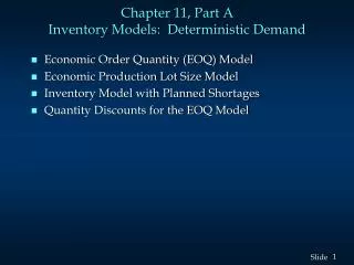
Chapter 11, Part A Inventory Models: Deterministic Demand
Chapter 11, Part A Inventory Models: Deterministic Demand. Economic Order Quantity (EOQ) Model Economic Production Lot Size Model Inventory Model with Planned Shortages Quantity Discounts for the EOQ Model. Inventory Models.

Chapter 11, Part A Inventory Models: Deterministic Demand
E N D
Presentation Transcript
Chapter 11, Part AInventory Models: Deterministic Demand • Economic Order Quantity (EOQ) Model • Economic Production Lot Size Model • Inventory Model with Planned Shortages • Quantity Discounts for the EOQ Model
Inventory Models • The study of inventory models is concerned with two basic questions: • How much should be ordered each time • When should the reordering occur • The objective is to minimize total variable cost over a specified time period (assumed to be annual in the following review).
Inventory Costs • Ordering cost -- salaries and expenses of processing an order, regardless of the order quantity • Holding cost -- usually a percentage of the value of the item assessed for keeping an item in inventory (including finance costs, insurance, security costs, taxes, warehouse overhead, and other related variable expenses) • Backorder cost -- costs associated with being out of stock when an item is demanded (including lost goodwill) • Purchase cost -- the actual price of the items • Other costs
Deterministic Models • The simplest inventory models assume demand and the other parameters of the problem to be deterministic and constant. • The deterministic models covered in this chapter are: • Economic order quantity (EOQ) • Economic production lot size • EOQ with planned shortages • EOQ with quantity discounts
Economic Order Quantity (EOQ) • The most basic of the deterministic inventory models is the economic order quantity (EOQ). • The variable costs in this model are annual holding cost and annual ordering cost. • For the EOQ, annual holding and ordering costs are equal.
Economic Order Quantity • Assumptions • Demand is constant throughout the year at D items per year. • Ordering cost is $Co per order. • Holding cost is $Ch per item in inventory per year. • Purchase cost per unit is constant (no quantity discount). • Delivery time (lead time) is constant. • Planned shortages are not permitted.
Economic Order Quantity • Formulas • Optimal order quantity: Q * = 2DCo/Ch • Number of orders per year: D/Q * • Time between orders (cycle time): Q */D years • Total annual cost: [(1/2)Q *Ch] + [DCo/Q *] (holding + ordering)
Example: Bart’s Barometer Business • Economic Order Quantity Model Bart's Barometer Business (BBB) is a retail outlet which deals exclusively with weather equipment. Currently BBB is trying to decide on an inventory and reorder policy for home barometers. Barometers cost BBB $50 each and demand is about 500 per year distributed fairly evenly throughout the year. Reordering costs are $80 per order and holding costs are figured at 20% of the cost of the item. BBB is open 300 days a year (6 days a week and closed two weeks in August). Lead time is 60 working days.
Example: Bart’s Barometer Business • Total Variable Cost Model Total Costs = (Holding Cost) + (Ordering Cost) TC = [Ch(Q/2)] + [Co(D/Q)] = [.2(50)(Q/2)] + [80(500/Q)] = 5Q + (40,000/Q)
Example: Bart’s Barometer Business • Optimal Reorder Quantity Q * = 2DCo /Ch = 2(500)(80)/10 = 89.44 90 • Optimal Reorder Point Lead time is m = 60 days and daily demand is d = 500/300 or 1.667. Thus the reorder point r = (1.667)(60) = 100. Bart should reorder 90 barometers when his inventory position reaches 100 (that is 10 on hand and one outstanding order).
Example: Bart’s Barometer Business • Number of Orders Per Year Number of reorder times per year = (500/90) = 5.56 or once every (300/5.56) = 54 working days (about every 9 weeks). • Total Annual Variable Cost TC = 5(90) + (40,000/90) = 450 + 444 = $894.
Example: Bart’s Barometer Business We’ll now use a spreadsheet to implement the Economic Order Quantity model. We’ll confirm our earlier calculations for Bart’s problem and perform some sensitivity analysis. This spreadsheet can be modified to accommodate other inventory models presented in this chapter.
Example: Bart’s Barometer Business • Partial Spreadsheet with Input Data
Example: Bart’s Barometer Business • Partial Spreadsheet Showing Formulas for Output
Example: Bart’s Barometer Business • Partial Spreadsheet Showing Output
Example: Bart’s Barometer Business • Summary of Spreadsheet Results • A 16.15% negative deviation from the EOQ resulted in only a 1.55% increase in the Total Annual Cost. • Annual Holding Cost and Annual Ordering Cost are no longer equal. • The Reorder Point is not affected, in this model, by a change in the Order Quantity.
Economic Production Lot Size • The economic production lot size model is a variation of the basic EOQ model. • A replenishment order is not received in one lump sum as it is in the basic EOQ model. • Inventory is replenished gradually as the order is produced (which requires the production rate to be greater than the demand rate). • This model's variable costs are annual holding cost and annual set-up cost (equivalent to ordering cost). • For the optimal lot size, annual holding and set-up costs are equal.
Economic Production Lot Size • Assumptions • Demand occurs at a constant rate of D items per year. • Production rate is P items per year (and P > D ). • Set-up cost: $Co per run. • Holding cost: $Ch per item in inventory per year. • Purchase cost per unit is constant (no quantity discount). • Set-up time (lead time) is constant. • Planned shortages are not permitted.
Economic Production Lot Size • Formulas • Optimal production lot-size: Q * = 2DCo /[(1-D/P )Ch] • Number of production runs per year: D/Q * • Time between set-ups (cycle time): Q */D years • Total annual cost: [(1/2)(1-D/P )Q *Ch] + [DCo/Q *] (holding + ordering)
Example: Non-Slip Tile Co. • Economic Production Lot Size Model Non-Slip Tile Company (NST) has been using production runs of 100,000 tiles, 10 times per year to meet the demand of 1,000,000 tiles annually. The set-up cost is $5,000 per run and holding cost is estimated at 10% of the manufacturing cost of $1 per tile. The production capacity of the machine is 500,000 tiles per month. The factory is open 365 days per year.
Example: Non-Slip Tile Co. • Total Annual Variable Cost Model This is an economic production lot size problem with D = 1,000,000, P = 6,000,000, Ch = .10, Co = 5,000 TC = (Holding Costs) + (Set-Up Costs) = [Ch(Q/2)(1 - D/P )] + [DCo/Q] = .04167Q + 5,000,000,000/Q
Example: Non-Slip Tile Co. • Optimal Production Lot Size Q * = 2DCo/[(1 -D/P )Ch] = 2(1,000,000)(5,000) /[(.1)(1 - 1/6)] = 346,410 • Number of Production Runs Per Year D/Q * = 2.89 times per year.
Example: Non-Slip Tile Co. • Total Annual Variable Cost How much is NST losing annually by using their present production schedule? Optimal TC = .04167(346,410) + 5,000,000,000/346,410 = $28,868 Current TC = .04167(100,000) + 5,000,000,000/100,000 = $54,167 Difference = 54,167 - 28,868 = $25,299
Example: Non-Slip Tile Co. • Idle Time Between Production Runs There are 2.89 cycles per year. Thus, each cycle lasts (365/2.89) = 126.3 days. The time to produce 346,410 per run = (346,410/6,000,000)365 = 21.1 days. Thus, the machine is idle for: 126.3 - 21.1 = 105.2 days between runs.
Example: Non-Slip Tile Co. • Maximum Inventory Current Policy: Maximum inventory = (1-D/P )Q * = (1-1/6)100,000 83,333 Optimal Policy: Maximum inventory = (1-1/6)346,410 = 288,675 • Machine Utilization Machine is producing D/P = 1/6 of the time.
EOQ with Planned Shortages • With the EOQ with planned shortages model, a replenishment order does not arrive at or before the inventory position drops to zero. • Shortages occur until a predetermined backorder quantity is reached, at which time the replenishment order arrives. • The variable costs in this model are annual holding, backorder, and ordering. • For the optimal order and backorder quantity combination, the sum of the annual holding and backordering costs equals the annual ordering cost.
EOQ with Planned Shortages • Assumptions • Demand occurs at a constant rate of D items/year. • Ordering cost: $Co per order. • Holding cost: $Ch per item in inventory per year. • Backorder cost: $Cb per item backordered per year. • Purchase cost per unit is constant (no qnty. discount). • Set-up time (lead time) is constant. • Planned shortages are permitted (backordered demand units are withdrawn from a replenishment order when it is delivered).
EOQ with Planned Shortages • Formulas • Optimal order quantity: Q * = 2DCo/Ch (Ch+Cb )/Cb • Maximum number of backorders: S * = Q *(Ch/(Ch+Cb)) • Number of orders per year: D/Q * • Time between orders (cycle time): Q */D years • Total annual cost: [Ch(Q *-S *)2/2Q *] + [DCo/Q *] + [S *2Cb/2Q *] (holding + ordering + backordering)
Example: Hervis Rent-a-Car • EOQ with Planned Shortages Model Hervis Rent-a-Car has a fleet of 2,500 Rockets serving the Los Angeles area. All Rockets are maintained at a central garage. On the average, eight Rockets per month require a new engine. Engines cost $850 each. There is also a $120 order cost (independent of the number of engines ordered). Hervis has an annual holding cost rate of 30% on engines. It takes two weeks to obtain the engines after they are ordered. For each week a car is out of service, Hervis loses $40 profit.
Example: Hervis Rent-a-Car • Optimal Order Policy D = 8 x 12 = 96; Co = $120; Ch = .30(850) = $255; Cb = 40 x 52 = $2080 Q * = 2DCo/Ch (Ch + Cb)/Cb = 2(96)(120)/255 x (255+2080)/2080 = 10.07 10 S * = Q *(Ch/(Ch+Cb)) = 10(255/(255+2080)) = 1.09 1
Example: Hervis Rent-a-Car • Optimal Order Policy (continued) Demand is 8 per month or 2 per week. Since lead time is 2 weeks, lead time demand is 4. Thus, since the optimal policy is to order 10 to arrive when there is one backorder, the order should be placed when there are 3 engines remaining in inventory.
Example: Hervis Rent-a-Car • Stockout: When and How Long How many days after receiving an order does Hervis run out of engines? How long is Hervis without any engines per cycle? ---------------------------- Inventory exists for Cb/(Cb+Ch) = 2080/(255+2080) = .8908 of the order cycle. (Note, (Q *-S *)/Q * = .8908 also, before Q * and S * are rounded.) An order cycle is Q */D = .1049 years = 38.3 days. Thus, Hervis runs out of engines .8908(38.3) = 34 days after receiving an order. Hervis is out of stock for approximately 38 - 34 = 4 days.
EOQ with Quantity Discounts • The EOQ with quantity discounts model is applicable where a supplier offers a lower purchase cost when an item is ordered in larger quantities. • This model's variable costs are annual holding, ordering and purchase costs. • For the optimal order quantity, the annual holding and ordering costs are not necessarily equal.
EOQ with Quantity Discounts • Assumptions • Demand occurs at a constant rate of D items/year. • Ordering Cost is $Co per order. • Holding Cost is $Ch = $CiI per item in inventory per year (note holding cost is based on the cost of the item, Ci). • Purchase Cost is $C1 per item if the quantity ordered is between 0 and x1, $C2 if the order quantity is between x1 and x2 , etc. • Delivery time (lead time) is constant. • Planned shortages are not permitted.
EOQ with Quantity Discounts • Formulas • Optimal order quantity: the procedure for determining Q * will be demonstrated • Number of orders per year: D/Q * • Time between orders (cycle time): Q */D years • Total annual cost: [(1/2)Q *Ch] + [DCo/Q *] + DC (holding + ordering + purchase)
Example: Nick's Camera Shop • EOQ with Quantity Discounts Model Nick's Camera Shop carries Zodiac instant print film. The film normally costs Nick $3.20 per roll, and he sells it for $5.25. Zodiac film has a shelf life of 18 months. Nick's average sales are 21 rolls per week. His annual inventory holding cost rate is 25% and it costs Nick $20 to place an order with Zodiac. If Zodiac offers a 7% discount on orders of 400 rolls or more, a 10% discount for 900 rolls or more, and a 15% discount for 2000 rolls or more, determine Nick's optimal order quantity. -------------------- D = 21(52) = 1092; Ch = .25(Ci); Co = 20
Example: Nick's Camera Shop • Unit-Prices’ Economical, Feasible Order Quantities • For C4 = .85(3.20) = $2.72 To receive a 15% discount Nick must order at least 2,000 rolls. Unfortunately, the film's shelf life is 18 months. The demand in 18 months (78 weeks) is 78 X 21 = 1638 rolls of film. If he ordered 2,000 rolls he would have to scrap 372 of them. This would cost more than the 15% discount would save.
Example: Nick's Camera Shop • Unit-Prices’ Economical, Feasible Order Quantities • For C3 = .90(3.20) = $2.88 Q3* = 2DCo/Ch = 2(1092)(20)/[.25(2.88)] = 246.31 (not feasible) The most economical, feasible quantity for C3 is 900. • For C2 = .93(3.20) = $2.976 Q2* = 2DCo/Ch = 2(1092)(20)/[.25(2.976)] = 242.30 (not feasible) The most economical, feasible quantity for C2 is 400.
Example: Nick's Camera Shop • Unit-Prices’ Economical, Feasible Order Quantities • For C1 = 1.00(3.20) = $3.20 Q1* = 2DCo/Ch = 2(1092)(20)/.25(3.20) = 233.67 (feasible) When we reach a computedQ that is feasible we stop computing Q's. (In this problem we have no more to compute anyway.)
Example: Nick's Camera Shop • Total Cost Comparison Compute the total cost for the most economical, feasible order quantity in each price category for which a Q * was computed. TCi = (1/2)(Qi*Ch) + (DCo/Qi*) + DCi TC3 = (1/2)(900)(.72) +((1092)(20)/900)+(1092)(2.88) = 3493 TC2 = (1/2)(400)(.744)+((1092)(20)/400)+(1092)(2.976) = 3453 TC1 = (1/2)(234)(.80) +((1092)(20)/234)+(1092)(3.20) = 3681 Comparing the total costs for 234, 400 and 900, the lowest total annual cost is $3453. Nick should order 400 rolls at a time.