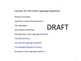
Lecture 16: The Euler-Lagrange Equations

1. Lecture 16: The Euler-Lagrange Equations Review of energies Geometric constraints (holonomic) DRAFT The Lagrangian Generalized coordinates Homogeneous Euler-Lagrange equations Generalized forces Forced Euler-Lagrange equations The Rayleigh dissipation function Dissipative Euler-Lagrange equations

2. We won’t get through it all today

3. By the way . . . As you’ve probably noticed simply reading the slides on the website is not enough You need to ask questions in class as the presentation slides by We’re going to do a lot today and some of it is pretty complicated Don’t let it get away from you

4. And Please turn in your Mathematica/Matlab work with your homework!

5. ENERGY kinetic energy potential energy gravity spring

6. SIMPLE UNCONSTRAINED SYSTEMS

7. SIMPLE PENDULUM q m

8. FIGURE 3.1 k1 k3 k2 m1 m2 y1 y2

9. TWO D MOTION (SMALL) OF A MASS z y IF y and z are small

10. CONSTRAINED MOTION We need as many variables as there are degrees of freedom and NO more We can often write down the energies without reference to constraints and then we have to apply the constraints before we can go on to analysis This is often a very good thing to do!

11. OVERHEAD CRANE y1, f1 M but so q m (y2, z2)

12. DOUBLE PENDULUM q1 m1 (y1, z1) There are six variables in the figure four variables in the energy expressions and but two degrees of freedom q2 m2 (y2, z2) We probably want to use the angles as our two independent variables

13. z geometric constraint y differentiate q1 m1 (y1, z1) substitute and simplify q2 m2 (y2, z2)

14. Yes, the energies are full of trigonometric functions and cross products This is OK. We cannot linearize until we have differential equations! We will always want to find the full nonlinear equations and then worry about linearization On to a general formalism

15. GENERALIZED COORDINATE FORMALISM We need as many coordinates as there are degrees of freedom no more, no fewer It is traditional to name them q1, q2, etc. For the overhead crane we can put y1 = q1 and q = q2 For the double pendulum we can put q1 = q1 and q2 = q2

16. The energies in terms of the generalized coordinates Note the special form of T

17. The LagrangianL = T - V The homogeneous Euler-Lagrange equations These are a set of second order equations, one for each degree of freedom We use them instead of the laboriously constructed equations from the FBDs

18. The process 1. Find T and V as easily as you can 2. Apply geometric constraints to get to N coordinates 3. Assign generalized coordinates 4. Define the Lagrangian

19. 5. Differentiate the Lagrangian with respect to the derivative of the first generalized coordinate 6. Differentiate that result with respect to time 7. Differentiate the Lagrangian with respect to the same generalized coordinate 8. Subtract that and set the result equal to zero Repeat until you have done all the coordinates

20. Some clarifications The partial derivative picks out only the variable chosen — here only explicit appearances of q1 OR its derivative The total derivative requires you to use the chain rule Apply this to the overhead crane

21. OVERHEAD CRANE y1, f1 M but so q m (y2, z2)

22. OVERHEAD CRANE y1, f1 Assign M Steps 1-4 lead us to q m (y2, z2)

23. For q1

24. For q2

25. The governing equations are then Put the physical variables back so it looks more familiar

26. Linearize (in two steps) Step one Step two: drop squares and higher products of the angles and their derivatives Final linear equations

27. We can find the natural frequencies of this system in the usual way There’s no damping, so we can seek harmonic solutions We can see from 8a that one of the frequencies will be zero and it represents motion of the cart with the pendulum fixed But let’s look at this more formally

28. Convert to matrix form The determinant simplifies to The nonzero frequency is the square root of

29. We can find the zero mode shape by inspection The other is which we can demonstrate The first row

30. The second row Substitute for w2 and simplify

31. The second motion has the cart moving in one direction and the pendulum moving in the opposite direction and the relative motion depends on the relative masses

32. Problem 68 Define as many coordinates as you like to make energies easy z2 z1 z1 and z2 for potential energy z z and q for kinetic energy q center of mass We’ll take this slowly to see how we ought to think

33. QUESTIONS? Let’s apply this to Problem 68, which we beat to death Tuesday evening

34. Kinetic Energy z center of mass y Tacit assumption: y is fixed

35. z center of mass z1 z2 y Tacit assumption: q remains small enough that sideways motion of the spring may be neglected

36. We have four coordinates and want only two I like z and q(and T is already in terms of these) Apply constraints to the potential energy

37. That can be simplified, and I’ll do that as I combine T and V to get L I can use z as q1 and q as q2, and I don’t need to do the specific substitution Now we can go through steps 5-8 for each of the variables

38. For q1

39. For q2

40. We can linearize the two equations

41. Seek harmonic solutions (which we can do because there is no damping) Replace the double dot by –w2 Write this in matrix form

42. The determinant is which expands to roots are as in the back of the book

43. As an aside it is not really a standard matrix eigenvalue problem as written because the w2 is multiplied by things We can clear those to make a standard eigenvalue problem (Note the change of angle variable.) Rewrite as The eigenvalues of this matrix will give the result we seek

44. Mathematica can find the eigenvalues (multiply by k/m) and the eigenvectors same as we got the first time high frequency is rotation low frequency is more up & down

45. We can do an initial value problem The homogeneous solution in terms of eigenvectors and eigenfunctions The initial conditions Substitute

46. The eigenvectors are real, so the complex conjugate notation is a mere formality Mathematica can do the algebra for us the coefficients the response

47. The modes are coupled If we look at the normalized eigenvectors the higher frequency is dominated by rotation the lower frequency is dominated (to a lesser extent) by up and down motion We can see this if we plot the results of the initial value problem

48. vertical motion rotational motion

49. vertical motion rotational motion

50. What did we do for both problems? What will we do for future problems?