MD5
MD5. MD5. Message Digest 5 Strengthened version of MD4 Significant differences from MD4 are 4 rounds, 64 steps (MD4 has 3 rounds, 48 steps) Unique additive constant each step Round function less symmetric than MD4 Each step adds result of previous step


MD5
E N D
Presentation Transcript
MD5 MD5 1
MD5 • Message Digest 5 • Strengthened version of MD4 • Significant differences from MD4 are • 4 rounds, 64 steps (MD4 has 3 rounds, 48 steps) • Unique additive constant each step • Round function less symmetric than MD4 • Each step adds result of previous step • Order that input words accessed varies more • Shift amounts in each round are “optimized” MD5 2
MD5 Algorithm • For 32-bit words A,B,C, define F(A,B,C) = (A B) (A C) G(A,B,C) = (A C) (B C) H(A,B,C) = A B C I(A,B,C) = B (A C) • Where , , , are AND, OR, NOT, XOR, respectively • Note that G “less symmetric” than in MD4 MD5 3
MD5 Algorithm MD5 4
MD5 Algorithm • Round 0: Steps 0 thru 15, uses F function • Round 1: Steps 16 thru 31, uses G function • Round 2: Steps 32 thru 47, uses H function • Round 3: Steps 48 thru 63, uses I function MD5 5
MD5: One Step • Where MD5 6
MD5 Notation • Let MD5i…j(A,B,C,D,M) be steps i thru j • “Initial value” (A,B,C,D) at i, message M • Note that MD50…63(IV,M) h(M) • Due to padding and final transformation • Let f(IV,M) = (Q60,Q63,Q62,Q61) + IV • Where “+” is addition mod 232 per 32-bit word • Then f is the MD5 compression function MD5 7
MD5 Compression Function • Let M = (M0,M1), each Mi is 512 bits • Then h(M) = f(f(IV,M0),M1) • Assuming M includes padding • That is, f(IV,M0) acts as “IV” for M1 • Can be extended to any number of Mi • Merkle-Damgard construction • Used in MD4 and many hash functions MD5 8
MD5 Attack: History • Dobbertin “almost” able to break MD5 using his MD4 attack (ca 1996) • Showed that MD5 might be vulnerable • In 2004, Wang published one MD5 collision • No explanation of method was given • Based on one collision, Wang’s method was reverse engineered by Australian team • Ironically, this reverse engineering work has been primary source to improve Wang’s attack MD5 9
MD5 Attack: Overview • Determine two 1024-bit messages • M = (M0,M1) and M = (M0,M1) • So that MD5 hashes are the same • That is, a collision attack • Attack is efficient • Many improvements to Wang’s original approach • Note that • Each Mi and Mi is a 512-bit block • Each block is 16 words, 32 bits/word MD5 10
MD5 Attack: Overview • Determine two 1024-bit messages • M = (M0,M1) and M = (M0,M1) • So that MD5 hashes are the same • That is, a collision attack • A differential cryptanalysis attack • Idea is to use first block to generate desired “IV” for 2nd block • Can be viewed as a “chosen IV” attack MD5 11
A Precise Differential • Most differential attacks use XOR or modular subtraction for difference • These are not sufficient for MD5 • Wang proposed • A “kind of precise differential” • More informative than XOR and modular subtraction combined MD5 12
A Precise Differential • Consider bytes y = 00010101 and y = 00000101 z = 00100101 and z = 00010101 • Note that y y = z z = 00010000 = 24 • Then wrt modular subtraction, these pairs are indistinguishable • In this case, XOR distinguishes the pairs y y = 00010000 z z = 00110000 MD5 13
A Precise Differential • Modular subtraction and XOR is not enough information! • Let y = (y0,y1,…,y7) and y = (y0,y1,…,y7) • Want to distinguish between, say, y3=0, y3=1 and y3=1, y3=0 • Use a signed difference, y • Denote yi=1, yi=0 as “+” • Denote yi=0, yi=1 as “” • Denote yi=yi as “.” MD5 14
A Precise Differential • Consider bytes z = 10100101 and z = 10010101 • Then z is “..+-....” • Note that both XOR and modular difference can be derived from z • Also note same given by pairs x = 10100101 and x = 10010101 y = 10100101 and y = 10010101 MD5 15
A Precise Differential • Properties of Wang’s signed differential • More restrictive than XOR or modular difference • Provides greater “control” during attack • But not too restrictive • Many pairs satisfy a given value • Ideal balance of control and freedom MD5 16
Wang’s Attack • Next, we outline Wang’s attack • On part theory and one part computation • Overall attack splits into 4 steps • More details follow • Then discuss reverse engineering of Wang’s attack • Finally, consider whether attack is a practical concern or not MD5 17
Wang’s Attack • Somewhat ad hoc • Consider input and output differences • Input differences • Applies to messages M and M • Use modular difference • Output differences • Applies to intermediate values, Qi and Qi • Use Wang’s signed difference MD5 18
Wang vs Dobbertin • Dobbertin’s MD4 attack • Input differentials specified • Equation solving is main part of attack • Wang’s MD5 attack • More of a “pure” differential attack • Specify input differences • Tabulate output differences • Force some output differences to hold • Unforced differences satisfied probabilistically MD5 19
Wang’s Attack: Step 1 • Specify input differential pattern • Must “behave nicely” in later rounds • These differentials are given below • Modular difference used for inputs • Only need to specify M • Then M is determined by differential MD5 20
Wang’s Attack: Step 2 • Specify output differential pattern • Must “behave nicely” in early rounds • That is, easily satisfied in early rounds • Restrictive signed difference used • Most mysterious part of attack • Wang used “intuitive” approach • Only 1 such pattern known (Wang’s) MD5 21
Wang’s Attack: Step 3 • Derive set of sufficient conditions • Using differential patterns • If these conditions are all met • Differential patterns hold • Therefore, we obtain a collision MD5 22
Wang’s Attack: Step 4 • Computational phase • Must find pair of 1024-bit messages that satisfy all conditions in step 3 • Messages: M = (M0,M1) and M = (M0,M1) • Deterministically satisfy as many conditions as possible • Any remaining conditions must be satisfied probabilistically • Number of such conditions gis expected work MD5 23
Wang’s Attack: Step 4 • Computational phase: • Generate random 512-bit M0 • Use single-step modification to force some conditions in early steps to hold • Use multi-step modification to force some conditions in middle steps to hold • Check all remaining conditions—if all hold then have desired M0, else goto b) • Follow similar procedure to find M1 • Compute M0 and M1 (easy) and collision! MD5 24
Wang’s Attack: Work Factor • Work is dominated by finding M0 • Work determined by number of probabilistic conditions • Work is on the order of 2n where n is number of such conditions • Wang’s original attack: n > 40 • Hours on a supercomputer • Best as of today, about n = 32.25 • Less than 2 minutes on a PC MD5 25
Wang’s Differentials • Input and output differentials • Notation: “+” over n for 2n and “” for 2n • For example: • Consider 2-block message: h(M0,M1) • Notation: IV = (A,B,C,D) • Denote “IV” for M1 as IV1 (and IV1 for M1) • Then IV1 = (Q60,Q63,Q62,Q61) + (A,B,C,D) • Where Qi are outputs when hashing M0 • Let h = h(M0,M1) and h = h(M0,M1) MD5 26
Wang’s Input Differential • Required input differentials M0 = M0 M0 = (0,0,0,0,231,0,0,0,0,0,0,215,0,0,231,0) M1 = M1 M1 = (0,0,0,0,231,0,0,0,0,0,0,215,0,0,231,0) • Note: M0 and M0 differ only in words 4, 11 and 14 • Note: M1 and M1 differ only in words 4, 11 and 14 • Same differences except in word 11 • Also required that IV1 = IV1 IV1 = (231, 225 + 231, 225 + 231, 225 + 231) • Goal is to obtain h = h h = (0,0,0,0) MD5 27
Wang’s Output Differential • Required output differentials • Part of M0 differential table: • Qi are outputs for M0 • Wj are input (modular) differences • Output is output modular difference • Output is output signed (“precise”) difference MD5 28
Derivation of Differentials? • Where do differentials come from? • “Intuitive”, “done by hand”, etc. • Input differences are fairly reasonable • Output differences are more mysterious • We briefly consider history of MD5 attacks • Then reverse engineering of Wang’s method • None of this is entirely satisfactory… MD5 29
History of MD5 Attacks • Dobbertin tried his MD4 approach • Modular differences and equation solving • No true collision obtained, but did highlight potential weaknesses • Chabaud and Joux • Use XOR differences • Approximate nonlinearity by XOR (like in linear cryptanalysis) • Had success against SHA-0 MD5 30
History of MD5 Attacks • Wang’s attack • Modular differences for inputs • Signed differential for outputs • Gives more control over outputs and actual step functions, not approximations • Also, uses 2 blocks, so second block is essentially “chosen IV” attack • Wang’s magic lies in differential patterns • How were these chosen? MD5 31
Daum’s Insight • Wang’s attack could be “expected” to work against MD-like hash with 3 rounds • Input differential forces last round conditions • Single-step modification forces 1st round • Multi-step modifications forces 2nd round • But MD5 has 4 rounds! • A special property of MD5 is exploited: • Output difference of 231 “propagated from step to step with probability 1 in the 3rd round and with probability 1/2” in most of 4th round MD5 32
Wang’s Differentials • No known method for automatically generating useful MD5 differentials • Daum: build tree of difference patterns • Include both input and output differences • Prune low probability paths from tree • Connect “inner collisions”, etc. • However, Wang’s differentials are only useful ones known today MD5 33
Reverse EngineeringWang’s Attack • Based on 1 published MD5 collision • Computed intermediate values • Examined modular, XOR, signed difference • Uncovered many aspects of attack • Resulted in computational improvements • Overall, an impressive piece of work! MD5 34
Conditions • For first round, define Tj = F(Qj1,Qj2,Qj3) + Qj4+ Kj + Wj Rj = Tj <<< sj Qj = Qj1+ Rj • Initial values: (Q4,Q3,Q2,Q1) • This is equivalent to previous notation MD5 35
Conditions • Let be modular difference: X =X X • Then Tj = Fj1+Qj4+Wj Rj ≈ (Tj) <<< sj Qj = Qj1+ Rj • Where Fj = F(Qj,Qj1,Qj2) F(Qj,Qj1,Qj2) • The Rjequation holds with high probability • Tabulated Qj, Fj, Tj, and Rjfor all j MD5 36
Conditions • Derive conditions on Tj and Qj that ensure known differential path holds • Conditions on Tj not used in original attack • More efficient recent attacks do use these • Goal is to deterministically (or with high prob) satisfy as many conditions as possible • Reduces number of iterations needed MD5 37
T Conditions • Recall Tj = Fj1+Qj4+Wj Rj ≈ (Tj) <<< sj • Interaction of “” and “<<<” is tricky • Suppose T = 220 and T = 219 and s = 10 • Then (T) <<< s = (T T) <<< s = 229 and (T <<< s) = (T <<< s) (T <<< s) = 229 • In this example, “” and “<<<” commute MD5 38
T Conditions • Spse T = 222, T = 221 + 220 + 219, s = 10 • Then (T) <<< s = (T T) <<< s = 229 but (T <<< s) (T <<< s) = 229 + 1 • Here, “” and “<<<” do not commute • Negative numbers can be tricky MD5 39
T Conditions • If T and s are specified, conditions on T are implied by R = (T) <<< s • Can always force a “wrap around” in R • Can be little bit tricky due to non-commuting • Recall Tj = F(Qj1,Qj2,Qj3) + Qj4+ Kj + Wj • Given M, conditions on Tj can be checked • Better yet, want to select M so that many of the required T conditions hold MD5 40
T Conditions: Example • At step 5 of Wang’s collision: T5 = 219 + 211, Q4 = 26, Q5 = 231 + 223 26, s5 = 12 • Since Qj = Qj1+ Rj, it is easy to show thatR5 = Q5Q4 = 231 + 223 • We also have R5 ≈ (T5) <<< s5 • Implies conditions on anyT5 that satisfies Wang’s differentials! MD5 41
T Conditions: Example • From the previous slide: R5 = 231 + 223 = (T5) <<< 12 • Of course, the known T5 works:T5 = 219 + 211 • But, for example, T5 = 220 219 + 211, does not work, since rotation would “wrap around” • Implies there can be no 220 term in T5 • Complex condition to restrict borrows also needed • Bottom line: Can derive a set of conditions on Ts that ensure Wang’s differential path holds MD5 42
Output Conditions • Easier to check Q conditions than T • The Q are known as “outputs” • Actually, intermediate values in algorithm • Much easier to specify M so that Q conditions hold than T conditions • In attacks, Q conditions mostly used MD5 43
Output Conditions • Use signed differential, X • For example, if X = 0x02000020 and X = 0x80000000 then X is denoted “-.....+. ........ ........ ..+.....” • Also we must analyze round function: F(A,B,C) = (A B) (A C) • Bits of A choose between bits of B and C MD5 44
Output Conditions: Example • At step 4 of Wang’s collision: Q2 = Q3 = 0, Q4 = 26, F4 = 219 + 211 • From Q4 we have: Q4= 19 and Q4= 010…25 • Note that Q4 = Q4at all other bits MD5 45
Output Conditions: Example • From Q4 we have: Q4= 19 and Q4= 010…25 • Note that Q4 = Q4at all other bits • Bits 9,10,…,25 are “constant” bits of Q4 • All others are “non-constant” bits of Q4 • On constant bits, Q4 = Q4 and on non-constant bits, Q4Q4 MD5 46
Output Conditions: Example • Consider constant bits of Q4 • Since F4 = F(Q4,Q3,Q2), from defn of F • If Q4= 1j then F4 = Q3j and F4 = Q3j • If Q4= 0j then F4 = Q2j and F4 = Q2j • Then F4 = F4j for each constant bit j • From table, constant bits of Q4 are constant bits of F4 so no conditions on Q4 MD5 47
Output Conditions: Example • Consider non-constant bits of Q4 • Since F4 = F(Q4,Q3,Q2), from defn of F • If Q4= 1j then F4 = Q3j and F4 = Q2j • If Q4= 0j then F4 = Q2j and F4 = Q3j • Note that on bits 10,11,13,…,19,21,…,25 F4 = F4, Q4 = 1, Q4 = 0 F4 = Q2, F4 = Q3 • Since Q3 = Q3we have Q3 = Q210,11,13…19,21,,,25 MD5 48
Output Conditions: Example • Still need to consider bits 9,12,20 • See textbook • From step 4, we derive the following output conditions: Q4 = 010,,,25, Q4 = 19 Q3 = 112,20 Q2 = 012,20, Q2 = Q310,11,13…19,21,,,25 MD5 49
Conditions: Bottom Line • By reverse engineering one collision… • Able to deduce output conditions • If all of these are satisfied, we will obtain a collision • This analysis resulted in much more efficient implementations • All base on one known collision! MD5 50