Quantitative Analysis: Managerial Decision Tools and Case Studies
420 likes | 493 Vues
Explore the application of linear programming, game theory, queuing models, simulation, and decision theory in making profitable managerial decisions. Learn key concepts and case studies. Dive into linear and nonlinear programming, emphasizing the importance of models and the relationship between good decisions and outcomes. Discover in-depth insights into profit-maximizing linear programming problems. Enhance your knowledge and skills in quantitative analysis with real-life examples.

Quantitative Analysis: Managerial Decision Tools and Case Studies
E N D
Presentation Transcript
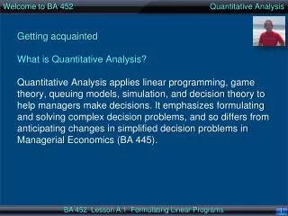
Welcome to BA 452 Quantitative Analysis Getting acquaintedWhat is Quantitative Analysis? Quantitative Analysis applies linear programming, game theory, queuing models, simulation, and decision theory to help managers make decisions. It emphasizes formulating and solving complex decision problems, and so differs from anticipating changes in simplified decision problems in Managerial Economics (BA 445).
Welcome to BA 452 Quantitative Analysis • Getting startedRead and bookmark the online course syllabus: • http://faculty.pepperdine.edu/jburke2/ba452/index.htm • It provides review questions for each lesson, and serves as a contract specifying our obligations to each other. In particular, note: • Linear Algebra (solve 2 equations for 2 variables), Calculus (take a derivative), and Introduction to Microeconomics are prerequisites, so review as needed. • Before each class meeting, download and read the PowerPoint lesson, as presented under the “Schedule” link. • Have a laptop with Management Scientist installed
Readings • Readings • For each lesson, you can use either the 12th edition or the 13th edition of the Anderson, Sweeney, Williams, … text. • For the first lesson in Part I (Lesson I.1), read Chapter 1
Overview • Overview
Quantitative Analysis • Quantitative Analysis
Quantitative Analysis • Overview • Quantitative Analysis applies linear and nonlinear programming, game theory, queuing models, simulation, and decision theory to help managers make profitable decisions.
Quantitative Analysis • The Harris Corporation • Major electronics company in Melbourne, FL. • Developed a computerized optimization-based production planning system. • Benefits: • On-time deliveries increased from 75% to 95%. • Expanded markets and market share. • Increased profits by $115 million annually.
Quantitative Analysis • KeyCorp • One of the largest bank holding companies in the US ($66.8 billion in assets). • Developed a system to measure branch activities, customer wait times, teller productivity. • Benefits: • Customer processing time reduced 53%. • Customer wait time reduced. • Cost savings of $98 million over 5 years.
Quantitative Analysis • NYNEX • Major telecommunications provider (16.5 million customers worldwide). • Developed optimization techniques for network planning. • Benefits: • Improved quality and reliability of network plans. • Savings of $33 million.
Quantitative Analysis • The definition of a model: • Models are simplified versions of the things they represent. • A useful model accurately represents the relevant or essential characteristics of the object or decision being studied. (Like a model airplane studied in a wind tunnel.)
Quantitative Analysis • Good decisions vs. good outcomes: • A structured, modeling approach to decision making helps make good decisions, but can’t guarantee good outcomes because of uncertainty (risk). • Life insurance is often a good decision, even when it turns out you do not die that year. • Other examples of good decisions with bad outcomes? • Betting your retirement savings on 17 Black in Roulette is often a bad decision, even if it turns out 17 Black wins. • Other examples of bad decisions with good outcomes?
Linear Programming • Linear Programming
Linear Programming Overview Linear Programming Problems in managerial applications often maximize profit, which equals revenue from outputs minus cost of inputs. Profit is a linear function of output and input decision variables, and linear constraints restrict permissible decision variables. A key lesson of quantitative analysis is exposure to the variety of profit-maximization linear-programming problems.
Linear Programming First, profit-maximization linear-programming problems can vary by whether outputs are fixed or variable, or whether inputs are fixed or variable: • In some problems, outputs are fixed (say, customers made reservations), so revenue is fixed and the objective of profit maximization reduces to the objective of cost minimization. • In other problems, inputs are fixed (say, airlines make short-run decisions about using their fixed stock of planes), so cost is fixed and the objective of profit maximization reduces to the objective of revenue maximization.
Linear Programming Second, problems can vary by whether available input resources are fixed or whether additional inputs may be bought: • In some problems, available input resources are fixed (say, firms make short-run decisions about how much labor to employ, from 0 up to a fixed maximum), so the problem is how to best allocate those resources to produce various outputs. • In other problems, additional inputs may be bought, so the problem is to balance the productivity of an input and its cost. • In still other problems, inputs can be either made or bought (say, Sony can either make parts for its televisions or buy parts).
Linear Programming Third, problems can vary by outputs and inputs are defined: • In some problems, outputs have different physical characteristics (say, Toyota produces both cars and trucks). • In other problems, outputs occur at different periods in time (say, Toyota produces cars for sale this year, and cars for sale next year). • In other problems, outputs occur at different locations (say, Toyota offers cars for sale in the US, and cars for sale in Japan). Likewise, inputs can have different physical characteristics, occur at different periods in time, and occur at different locations
Linear Programming • Many linear programming applications are interrelated, according to the following chart. For example, Assignment is a type of Transportation Problem, which in turn is a type of Transshipment Problem, which is a type of Resource Allocation Problem.
Linear Programming • Linear programming problems have constraints on pursuing the objective of maximization or minimization. • A feasible solution satisfies all the constraints. • An optimal solution (or optimum) is a feasible solution that results in the largest possible objective-function value when maximizing (or smallest when minimizing).
Linear Programming • In a linear-programming problem, the objective function and the constraints are linear. • Functions are linear when each variable appears in a separate term raised to the first power and is multiplied by a constant (which could be 0). • Thus 5x1 + 7x2 is a linear function, but 5x12 +7x1x2 is not. • Linear constraints (or, standard linear constraints) are linear functions that are restricted to be "less than or equal to", "equal to", or "greater than or equal to" a constant. • Thus 2x1 + 3x2< 19 is a linear constraint, but 2x1 + 3x2 < 19 and 2x1 + 3x1x2< 19 are not.
Linear Programming The three steps to linear programming: • Formulate the linear programming problem. • Solve the problem, using either graphical or computer analysis. • In BA 452 lectures, homeworks and exams, you will solve some simple LP problems graphically, for the purpose of introducing and better understanding the concepts. • In BA 452 lectures, homeworks and exams, you will solve other complex LP problems by any means possible, including using program and spreadsheet templates stored on your laptop. • Interpret the solution.
Linear Programming • Problem formulation (or modeling) is the translation of a verbal statement of a decision problem into a mathematical statement. • Here are guidelines for linear programming problem formulation: • Describe the objective. • Describe each constraint. • Define the decision variables. • Write the objective in terms of the decision variables. • Write the constraints in terms of the decision variables.
Resource Allocation • Resource Allocation
Resource Allocation Overview Resource Allocation Problems are Linear Programming Profit Maximization problems when available input resources are fixed. Resource Allocation Problems thus help production managers allocate various fixed resources (labor, machine use, storage space, …) to produce various outputs (cars, trucks, …) to maximize profit or minimize cost. The opportunity cost of the scarce resources used in manufacture define the maximum willingness to pay if additional inputs became available.
Resource Allocation Question: Iron Works, Inc. seeks to maximize profit by making two products from steel. • It just received this month's allocation of 19 pounds of steel. • It takes 2 pounds of steel to make a unit of product 1, and 3 pounds of steel to make a unit of product 2. • The physical plant has the capacity to make at most 6 units of product 1, and at most 8 units of total product (product 1 plus product 2). • Product 1 has unit profit 5, and product 2 has unit profit 7. Formulate the linear program to maximize profit.
Resource Allocation Answer: Here is a mathematical formulation of the objective. • Let x1 and x2 denote this month's production level of product 1 and product 2. • The total monthly profit = (profit per unit of product 1) x (monthly production of product 1) + (profit per unit of product 2) x (monthly production of product 2) = 5x1 + 7x2 • Maximize total monthly profit: Max 5x1 + 7x2
Resource Allocation Here is a mathematical formulation of constraints. • The total amount of steel used during monthly production = (steel used per unit of product 1) x (monthly production of product 1) + (steel used per unit of product 2) x (monthly production of product 2) = 2x1 + 3x2 • That quantity must be less than or equal to the allocated 19 pounds of steel (the inequality < in the constraint below assumes excess steel can be freely disposed; if disposal is impossible, then use equality =) : 2x1 + 3x2 < 19 • The constraint that the physical plant has the capacity to make at most 6 units of product 1 is formulated x1< 6 • The constraint that the physical plant has the capacity to make at most 8 units of total product (product 1 plus product 2) is x1 + x2 < 8
Resource Allocation Adding the non-negativity of production completes the formulation. Objective function Max 5x1 + 7x2 s.t. x1< 6 2x1 + 3x2< 19 x1 + x2< 8 x1> 0 and x2> 0 Standard constraints Non-negativity constraints “Max” means maximize, and “s.t.” means subject to.
Portfolio Selection • Portfolio Selection
Portfolio Selection Overview Portfolio Selection Problems help financial managers select specific investments (stocks, bonds, …) to generate returns to either maximize expected return or minimize risk. Constraints may restrict permissible investments by state laws or company policy, and restrict risk.
Portfolio Selection Question: Fidelity Investments manages funds for a variety of clients. The investment strategy is tailored to each client’s needs. For a new client, Fidelity has been authorized to invest up to $1.2 million in two funds: a stock fund and a money market fund. Each unit of the stock fund costs $50 and returns an expected 10% annually. Each unit of the money market fund costs $100 and returns an expected 4% annually.
Portfolio Selection The client wants to minimize risk subject to the expected annual income is at least $60,000. According to Fidelity’s risk measurement system, each unit invested in the stock fund has a risk index of 8, and each unit in the money market fund has index of 3. (A higher index indicates a riskier investment.) Fidelity’s client also specified that at least $300,000 be invested in the money market fund. Formulate the linear program to minimize the total risk index of the portfolio.
Portfolio Selection Answer: • Define decision variables: • S = number of units purchased in the stock fund • 50S are the dollars invested in the stock fund • 5S is the 10% return from the dollars invested in the stock fund • M = number of units purchased in the money market fund • 100M are the dollars invested in the money fund • 4M is the 4% return from the dollars invested in the money fund • Define objective: Minimize 8S + 3M • Define constraints: • 50S + 100M <1,200,000 (Funds available) • 5S + 4M >60,000 (Annual income) • M >3,000 (Minimum units in money market) • S, M > 0 (Non-negativity)
Resource Allocation with Machines • Resource Allocation with Machines
Resource Allocation with Machines Overview Resource Allocation Problems with Machines help production managers allocate specific resources (including machine use) to produce goods to either maximize profit or minimize cost. Machine use is measured in hours, just like labor use.
Resource Allocation with Machines Question: Engineered Plastic Components, Inc. makes plastic parts used in automobiles and computers. One of its major contracts involves the production of plastic printer cases for a computer company’s portable printers. The printer cases can be produced on two injection molding machines. The M-100 machine has a production capacity of 25 printer cases per hour, and the M-200 machine has a production capacity of 40 printer cases per hour. Both machines use the same chemical to produce the printer cases; the M-100 uses 40 pounds of raw material per hour, and the M-200 uses 50 pounds per hour.
Resource Allocation with Machines The computer company asked EPC to produce as many of the cases as possible during the upcoming week; it will pay $18 for each case. However, next week is a regularly scheduled vacation period for most of EPC’s production employees. During this time, annual maintenance is performed on all equipment. Because of the downtime for maintenance, the M-100 is only available for at most 15 hours, and the M-200 for at most 10 hours.
Resource Allocation with Machines The supplier of the chemical used in the production process informed EPC that a maximum of 1000 pounds of the chemical material will be available for next week’s production; the cost for this raw material is $6 per pound. In addition to the raw material cost, Jackson Hole estimates that the hourly cost of operating the M-100 and the M-200 are $50 and $75, respectively.
Resource Allocation with Machines However, because of the high setup cost on both machines, management requires that, if a machine is used at all, it must be used for at least 5 hours. Formulate the linear program to maximize profit. To simplify this problem, you may change the last constraints to read that each machine must be used for at least 5 hours. (Do you see the difference between “if a machine is used at all, it must be used for at least 5 hours” and “each machine must be used for at least 5 hours”.)
Resource Allocation with Machines Answer: • Define decision variables (assuming positive use of both machines; a general solution requires binary variables from Part II of the course): • M1 = number of hours spent on the M-100 machine • 25 M1 is the production of cases from the M-100 machine • 18(25) M1 is the revenue from production from the M-100 machine • 40 M1 is the raw material used by the M-100 machine • M2 = number of hours spent on the M-200 machine • 40 M2 is the production of cases from the M-200 machine • 18(40) M2 is the revenue from production from the M-200 machine • 50 M2 is the raw material used by the M-200 machine • Total revenue = 18(25) M1 + 18(40) M2 = 450 M1 + 720 M2 • Total cost = 6(40) M1 + 6(50) M2 + 50 M1 + 75 M2 = 290 M1 + 375 M2
Resource Allocation with Machines • Define objective: Maximize (profit = revenue-cost) 160 M1 + 345 M2 • Define constraints: • M1<15 (M-100 maximum) • M2<10 (M-200 maximum) • M1>5 (M-100 minimum) • M2>5 (M-200 minimum) • 40M1 + 50 M2<1000 (Raw Material) • M1, M2> 0
BA 452 Quantitative Analysis End of Lesson A.1