Download
1 / 31
310 likes | 478 Vues
Lecture Two. The rules for coding adjoint and the application of 3D variational method to radar data analysis. Jidong Gao jdgao@ou.edu November 2006 Center for Analysis and Prediction of Storms University of Oklahoma. What is the adjoint?

E N D
Lecture Two The rules for coding adjoint and the application of 3D variational method to radar data analysis Jidong Gaojdgao@ou.eduNovember 2006 Center for Analysis and Prediction of Storms University of Oklahoma
What is the adjoint? • It’s only a mathematical tool to help you to get the gradient of the cost function. • In Errico (1997) “What is an adjoint model?”, It is said “…the adjoint is used as a tool for efficiently determining the optimal solutions. Without this tool, the (4D) optimization problem (including minimization and maximization) could not be solved in a reasonable time for application to real-time forecasting”. This is a good statement. Then what does it mean exactly?
The adjoint • For a 3D cost function defined as • It’s gradient w.r.t. x is • It involves the HT operator and associated calculation. This HT is the ‘adjoint’ of H. • For a problem of small size, one can explicitly express H in a matrix form and perform explicit transpose operation and associated caculations. For a large problem, this is unrealistic and the sparseness of H also makes it unnecessary. • Here, the ‘adjoint’ coding technique comes to the rescue.
Mathematical definition of adjoint: • For any linear forward operator: X=LY, the adjoint code will be: Yad=LTX • A simple example for coding adjoint: forward code: do i = 1, N-1 x(i)=x(i)+a*y(i+1) end do input: xin, yin; output: xout the adjoint code: do i = 1, N-1 ad_y(i+1)= a*ad_x(i) ad_x(i) = ad_x(i) end do input: ad_xin,; output: ad_xout, ad_yout. To verify the correctness of the adjoint code, you can calculate the following two terms: xin * ad_xout + yin *ad_yout xout *ad_xin They should be equal.
1D variational interpolation scheme y M=6 1 x N=12 A problem: Suppose we have M irregular “observations” of a sinusoidal function in y, we’d like to determine values at regular grid points from 1 to N that best represent the function. First guess: pink curve.
We can define a cost function, Subroutine FCN(N, T, F) ! subroutine calculating the cost function Implicit none Use module_const ! Include observational number m=6 Use module_pass ! Use this to pass forcing term forc(m) to gradient sub. !!!! and observation value Tob(6), and its location y(6). integer::N, i, j; real::T(N), J, temp ! T is the state vector defined as location vector x J = 0.0 do i=1,n J = J+0.5*(T(i)-Tb(i))**2 enddo do j=1, m i = max(1, min(n, int (y(j)/dx)+1) ) temp=T(i)*(x(i+1)-y(j))/dx+T(i+1)*(y(j)-x(i))/dx forc(j)= temp-Tob(j) J = J+0.5*forc(j) **2 end do return end
Calculation of cost function gradident • How to calculate the gradient? Its not straightforward, because of the reasons stated earlier, and because the cost function for obs. is the summation of innovation vector in obs. points, not in grid points. But when we do the minimization, it is the gradients of cost function with respect to the analysis variables at the grid points that are required. We can use the adjoint technique to solve this problem. The formulation for the gradient is, The second term on rhs transfers the gradient of the cost function from the obs points to the grid points. It can be coded using the adjoint technique. “Recipes for Adjoint Construction” by Giering and Kaminski 1998) offers a good tutorial. Linked to at the class web site.
Subroutine GRAD(N, t, G) Implicit none • Use module_const ! Include observational number m=6 • Use module_pass ! Use this to pass forc(6) from sub FCN • !!!! and observation value Tob(6), and its location y(6). • integer::N, i, j; real::T(N), J, temp G(:) = 0.0 • do j=1, m • i = max(1, min(n, int (y(j)/dx)+1) ) • G(i) = G(i) + 0.5*forc(j)*(x(j+1)-y(j))/dx • G(i+1)=G(i+1)+0.5*forc(j)*(y(j)-x(j))/dx • end do do i=1,N G(i)=G(i)+0.5*(T(i)-Tb(i)) end do • return; end
storm-scale phenomenon By storm-scale, we mean structures like these We will need to predict the structure and evolution of individual cells Spatial scale ~ few km Time scale ~ tens of mins For storms, radar is about the only obs platform!
Radar Data Assimilation The Radar Problem: Observe radial velocity and reflectivity, other dual-polarization variables. But NWP model, needs V, T, P, qv, qr etc for IC. Real wind v u r y x Radial Vr
NEXRAD Radar provides high spatial and temporal resolution observations Assimilation of these radar data into storm-resolving models is very important for the future of operational forecasting Here, I will provide an example using the 3DVAR method to do single-Doppler velocity retrieval
We are trying to retrieve 3-D wind vectors from single-Doppler observed reflectivity and radial velocity during a short time period. A cost-function is defined as follows: J=JB + JO + JE+ JD + JS JB, background field constraint, Jo, radial wind constraint, JE, observed tracer constraint (reflectivity), JD, 3-D anelastic mass continuity equation, JS, smoothness constraints.
1) Background field constraint background can be obtained from other data source. A nearby sounding is used here. 2) Jo, measures the difference between the analyzed radial velocity and the observed radial velocity: Vr is obtained by interpolating retrieved variables u,, v,and w from the grid to observation points, then projecting the winds to the radial direction.
Here u, v, and w are velocities to be retrieved. • 3) Observed tracer constraint defines relationship of retrieved variables u, v, w and observed tracerh in the simplified equation,
4) Anelastic mass continuity constraint JDimposes a weak anelastic mass conservation on the analyzed winds. 5) Smoothness constraint The spatial smoothness term is used to remove small -scale noise and improve the quality of analysis.
A single observation experiment, no other constraint horizontal slice at z=9km u-v vector, contour of u Vertical slice at y=42km, w contour
Same as above, adding JD, JE horizontal slice at z=9km u-v vector, contour of u Vertical slice at y=42km, w contour
Analysis of May 17, 1981 Arcadia Storm, with Cimarron Radar Z = 9 km Z = 500 m An analysis with the radial velocity obs. only, no bkgd or other constraints. We get the results as expected Z = 4.5 km
Real Radar Data Analysis Cimarron Radar, cont’dwith a vertical slice at j = 25
Z = 500 m Same as the above, but add JD, JE, but without JS Z = 9.0 km Z = 4.5 km
with bkgd, but without smoothness Z = 500 m Z = 4.5 km J = 25
SDVR-Retrieved Dual-Doppler A A B B Cima OK Norman,OK Norman, OK 16:34 CST, May 17th, 1981, Arcadia, OK storm • Wind vector at Z=500m. Shaded is observed reflectivity field.
SDVR-Retrieved Dual-Doppler Vertical slice through line A-B in the horizontal slice.
Comments • Single obs. tests illustrates the behavior of 3DVAR for the analysis of radial wind. • When applying 3dvar to radar data, smoothness constraints, or background error covariances, or filters must be used to properly spread the influence of data. • With all constraints used, we can obtain pretty good analysis of storm structure, otherwise we obtain only the radial wind component plus a uniform background field.
Possible future research • radar data - essential for storm-scale NWP • available radar data: • radial velocity • reflectivity • quantities from dual-polarization measurements, such as, differential reflectivity, differential phase shift, etc • vertical wind profiles • accumulated rainfall
Possible future research (con’d) • thinning of too dense data consistently with the resolution of the analyses • study of space- and time structure of biases between simulated and observed data for bias correction
Possible future research (con’d) • reflectivity is sensitive to cloud properties • simulation depends on clouds representation in model • Start from idealized study, to get simulated reflectivity from model itself • study of existing radar simulation models
Possible future research (con’d) • code tangent linear and adjoint of observation operator • functional 3DVar minimization • check speed and quality • simulate and assimilate single radar data • check how 3DVar corrects atmospheric fields
Possible future research (con’d) • study the impact of reflectivity assimilation to forecast • for different situations (front, strong convection...) • for different resolutions (10 km, 2.5 km) • check spin up
Thank You for your attention! Questions? Send email to: jdgao@ou.edu or visit Rm 4110