Download
1 / 55
550 likes | 657 Vues
Why take a systems approach to the complexity of the magnetosphere? Asks questions other approaches usually don’t ... ... so gets answers other approaches won’t. Nick Watkins British Antarctic Survey (NERC) Cambridge, UK nww@bas.ac.uk. ISSI Meeting 2012. Thank co-authors 1998-.

E N D
Why take a systems approach to the complexity of the magnetosphere?Asks questions other approaches usually don’t ...... so gets answers other approaches won’t ... Nick Watkins British Antarctic Survey (NERC) Cambridge, UK nww@bas.ac.uk ISSI Meeting 2012
Thank co-authors 1998- Gary Abel (BAS)Tom Chang (MIT)Sandra Chapman (Warwick) Gareth Chisham (BAS)Dan Credgington (BAS/UCL)Richard Dendy (Culham) Andy Edwards (BAS/DFO)Mervyn Freeman (BAS) Christian Franzke (BAS)John Greenhough (Warwick/Edinburgh) Bogdan Hnat (Warwick)Khurom Kiyani (Warwick)Dave Riley (BAS/Cambridge) Sam Rosenberg (BAS/Cambridge)Raul Sanchez (Oak Ridge) Sunny Tam (MIT/)
Some Reviews: Vassiliadis, Rev. Geophys., 2006Dudok de Wit, in Space Plasma Simulation, 2003Freeman and Watkins, Science, 2002Watkins, Nonlinear Proc. Geophys., 2002Chapman and Watkins, Space Sci. Rev., 2001 Watkins et al., JASTP, 2001 Klimas et al., JGR, 1996 Sharma, Rev. Geophys. (Supp.), 1995
Why take a (complex) systems approach ? ... & secondly, because complexity is itself a frontier of modern science (reaching out towards a “science of sciences” [Neil Johnson, “Two’s Company, Three’s Complexity”]) Not surprising: frontiers of 21st century physics include the very large, the very small, and the very complex (where physics meets geophysics, biology, economics, society ...)
Why take a (complex) systems approach ?... and exploits frontiers with & connections into other areas of physics in a natural unforced way ...
Complex, not “just” complicated Adapted from Rudolf Treumann “Warm” Few effective variables “Cold” Many independent variables “Hot” “Complex systems are those with many strongly interdependent variables. This excludes systems with only a few effective variables, the kind we meet in elementary dynamics. It also excludes systems with many independent variables; we learn how to deal with them in elementary statistical mechanics. Complexity appears where coupling is important, but doesn't freeze out most degrees of freedom”. Cosma Shalizi , “Physics Today” [ 2005]
“The Guardian” [ 2000] Obviously nonspecialists still want to know that these answers are useful ... ... examples are likelihood of an extreme event [Koons, 2001], return time to next peak [Choe et al., 2002], heating effect of an auroral index “burst” [Uritsky et al., 2001] and value of AE index ...
PDF of AE Watkins, NPG, 2002. 10 years AE (l), 6 months (r). Bilognormality noted in |AL| Vassiliadis et al, 1996; AE Consolini & de Michelis 1998.
Illustrate only 3 techniques ... Others at ISSI will cover state of the art techniques, I have chosen two linear ones that any physicist will be comfortable with: the power spectral density (PSD) & autocorrelation function (ACF) ... ... to preface a less familiar one. Burst (size and duration) measures introduced into space physics by Consolini (1997) and Takalo (1994), & directly inspired by SOC. At each stage will try to show how the extra info changes our perspective- & to “join the dots ...“- will advocate more of this process
... & 1 complex system ... Solar wind Ionosphere Magnetosphere Example of AE: 12 magnetometers, sensing ionospheric currents. Ultimately energy is turbulent SW...
solar wind magnetosphere flow Sun • magnetic pole equator Convection (DP2) • Mass, momentum and energy input from reconnection at solar wind - magnetosphere interface. • Plasma circulation from day to night over poles and from night to day around flanks. Courtesy Mervyn Freeman
solar wind magnetosphere Substorms (DP1) BANG! • Irregular, large-scale releases of energy in magnetotail -substorms. • Intense magnetic field-aligned currents accelerate particles to cause aurora. Courtesy Mervyn Freeman
How is AE defined ? Indices estimate auroral dissipation. viaupper (AU) & lower (AL) envelope of magnetic perturbations from 12 magnetometers underneath auroral electrojets. Total envelope (AE)=AU-AL
Fourier spectrum S(f) [Tsurutani] Note absence of the peak he was expecting-an LCR circuit-like resonance on substorm time scales O(2 hrs) ... and existence of ever increasing LF power rather than a flat white noise ... Low pass SW??? Tsurutani et al, GRL,1991
S(f) of d/dt AE A. Pulkkinen et al, JGR, 2006
Modelling HF spectrum ... • Ignoring LF component, NB quite a few ways to make an f--2 high frequency spectrum, e.g.: • A nonstationary Brownian random walk • addition of many random variables • - f--2 all the way down • A stationary Ornstein-Uhlenbeck process • relaxation of a white noise driven system • - LF is white, HF is f--2 , turnover set by correlation time (aka AR(1)) • A “random telegraph” [c.f. Jensen book; • Watkins et al, Fractals, 2001] • State changes: high to low at Poisson intervals
Correlation structure Example dataset: 4 days of AE by Shan, Hansen, Goertz & Smith GRL, 1991. Search for correlations motivated by search for low dimensional chaos-but good system measure outlives its first application
Autocorrelation Function Shan et al, op. cit. ACF is essentially same information as PSD presented differently-as function of lag, rather than S(f)
Does ACF stabilise [Takalo] ? After Takalo & Timonen, GRL,1994
Limit of ACF ACF stabilises on periods of a few weeks, as it should because 1/f spectrum is also repeatable ... ... BUT sum (terms of ACF) blows up as longer and longer periods studied-classic indicator of long range dependence- (LRD) aka “Joseph effect” [Mandelbrot]
Long Range Dependence ß=1 Illustrate using fractional Brownian motion, here is index of power spectral slope ß Courtesy Gary Abel ß=2
Models for LRD/Joseph effect: As before can model LRD using nonstationary but H-selfsimilar models, e.g. fractional Brownian motion ... ... Or stationary but not exactly H-selfsimilar ones ... ... So what’s this H-selfsimilarity then ?
Self-similarity(affinity) and H S. d. of differences grows with time separation as return probability P(0) shrinks Brownian walk: “the “normal” model of natural fluctuations …” Mandelbrot (1995)
Single exponent: H=J=1/2 σ~ J Return pdf ~ -H Courtesy Bogdan Hnat
LRD alters J (and ß), H no longer 1/2 ß=1 Courtesy Gary Abel ß=2
There is another route to H > ½: heavy-tailed jumps Consolini& De Michelis, 1998
“Noah”effect- heavy(ish) tails in ∆AE [Consolini] E.g.Chapman et al, NPG [2004] pdf of AE at 15 min Alpha-stable Lévy flight Courtesy Andy Edwards
Either/both LRD or heavy tails will make simple Brownian H=1/2 random walk unsuitable Complexity- in time series manifests via anomalous “burstiness”.Time series counterpart of anomalous transport .......may seem like another buzzword so ...
COFFEE Ballistic ~ t ?? blah ?! Blah Anomalous ~ t^H After a really good poster session, diffusive t^1/2
Spatiotemporal phenomena need spatiotemporal diagnostics We need complementary ways of probing this sort of data, & (in my view) NOT ONLYsimple toy models for insight-and calibration of the diagnostics-BUT ALSO intermediate complexity models (c.f. climate science) AND physical theories of burstiness. One probe is the sort of finite range scaling collapses that Sandra is talking about ...another is burst size/duration – I’ll talk about some toy models for understanding what these do ...
Multiscaling ??? σ Pdf of returns Return pdf and σ scale same way in top 3 plots (all auroral) but differently in bottom one (solar wind) Watkins et al, Space Science Reviews [2005]
Could an H-selfsimilar model still capture this ? [standard Lévy motion, sLm] and fBm, however, are far from exhausting the anomalies found in nature ... many phenomena exhibit both the Noah and Joseph effects and fail to be represented by either sLm or fBm ... One obvious bridge, fractional Lévy motion, is interesting mathematically, but has found no concrete use". – Mandelbrot, 1995.
Linear fractional stable motion LFSM X(t) as given in Stoev and Taqqu, Fractals [2004]. Standard model in stats less well known in physics than fBm etc. Parameters d (“Joseph”) and α (“Noah”) both contribute to H, the selfsimilarity exponent: Allows subdiffusive H to coexist with superdiffusive α. We have derived kinetic equation for this in Watkins et al., (PRE,2009).
Watkins et al [SSR, 2005] Modelling with LFSM
(q) vs q plot for LFSM: ß (i.e d) varying, fixed at 1.5 Watkins et al, [Space Sci. Rev., 2005] “Structure function” (generalised variogram) (q) if monofractal then: q Demonstration of known multi-affine, “pseudo multifractal” behaviour-extends effect in ordinary Levy motion (=2)
Replot SVD/SSA mode heirarchy Sitnov et al, PRE, 2001
A very bold postulate …[Bak, Tang & Wiesenfeld, ‘87-’88] “In fact, there is one area of physics where the relation between spatial and temporal power-law behaviour is well-established. At the critical point for continuous phase transitions, the correlation function for the order parameter decays spatially ... and temporally as [power laws] But in order to arrive at the critical point, one has to fine-tune an external control parameter such as the temperature or pressure, in contrast to the phenomena above [1/f noise, spatial fractals] which occur universally without any fine-tuning. The explanation is that open, extended, dissipative dynamical systems may go automatically to the critical state as long as they are driven slowly: the critical state is self-organised. We see fractals as snapshots of systems operating at the self-organised critical (SOC) state” - Bak and Chen, Physica D [1989]and “Fractals in Physics”
Avalanches as bursts ... BTW, PRE 1988
Amplitude Burst with integrated “size” s taken over blue area Threshold time Duration T Waiting Time ... motivated “burst” diagnostic Courtesy Mervyn Freeman Measure designed for activity series in sandpile models
Burst size [Consolini, 1997-98] AE burst size for 10 years (main), 1 year (inset). “Fractals-what you see is what you wait for ...”
Probability density T (min) Burst duration Method introduced by Takalo, 1993 (inset). Main plot Riley, unpublished 2000 for AE 1978-85 (cf Consolini, ‘99)
Durations: AU, AL & SW 1978-88 1995-98 Freeman et al, GRL, 2000
Bump in AE family not SW Method Consolini 1999 preprint; Freeman et. al., op. cit.
Freeman et al [PRE, 2000] Poynting flux bursts @ L1 P(s) P() P() P(T)
Bursts in random walk models • Showing work in progress: Reported partly in Watkins et al ( PRE, 2009), • See second talk at ISSI for details • Bursts show spatiotemporal connections-need such a process to model them-show LFSM-will also study multifractals e.g. p-model (Watkins et al, PRL, 2009).
Adapt recent work of Kearney and Majumdar [2005] : simple scaling even for Brownian bursts s ~T ’, P(s) ~ s with ’=3/2 and =-4/3 s Show example “calibration” simulations in Brownian (=2, =2, H=0.5) case, here s v (top)] –steps toward interesting size-duration scaling seen in AE by Uritsky et al, 2001 (right) s
It’s not all noise – new generation of dynamical models: Fokker Planck: Hnat et al, GRl, JGR, 2002-3Langevin: Pulkkinen et al, JGR, 2006. SDE: Anh et al, JGR, 2008 SDE: Rypdal and Rypdal, PRE, 2008 Integrate & fire : Freeman-Morley, GRL.
Conclusions Complexity nothing to be scared of-on contrary need for it can be seen even in investigations of early 1990s using very familiar methods-PSD and ACF. Results show evidence of spatiotemporal bursts and scaling-motivate the use of newer diagnostics. We are using simple models of burstiness to unpick what has already been seen and help join the dots-showed you some preliminary results. Will feed into dynamical models. Complements other methods you have seen/will see.
AL conditional PDF Ukhorskiy et al
Scaling in AE: Activity-lifetime Uritsky et al., [GRL] have measured the dependence of N( )= <AE(t+ )> -L a time averaged activity measure And P() = n ( )/ m A survival probability (with the n the number of events with duration T > ) on averaging time Repeated for solar wind, (different) scaling relations found