Download
1 / 53
530 likes | 1k Vues
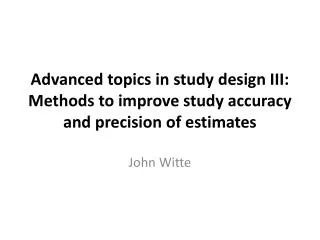
Advanced topics in study design III: Methods to improve study accuracy and precision of estimates. John Witte. Overview. Validity and Precision Bias Confounding Selection Bias Information Bias Improving Study Accuracy Matching Statistical Testing and Estimation.

E N D
Advanced topics in study design III: Methods to improve study accuracy and precision of estimates John Witte
Overview • Validity and Precision • Bias • Confounding • Selection Bias • Information Bias • Improving Study Accuracy • Matching • Statistical Testing and Estimation
1. Study Validity & Precision • A key goal in epi: estimation of effects with minimum error. • Sources of errors are systematic and random. • Systematic error (bias) affects the validity of a study. • A valid estimate is one that is expected to equal the true parameter value; various biases detract from validity. • Random variation reflects a lack of precision (e.g., wide CI). • Statistical precision = 1 / random variation • Improve precision by increasing • sample size (to a point) • size efficiency (i.e., maximizing amount of “information” per individual; example: selecting the same number of cases & controls).
Example: Validity versus Precision • Assume that two people are playing darts, with the goal of getting one’s throws as close as possible to the bull’s-eye. • Player 1’s aim is unbiased (valid), but their darts generally land in the outer regions of the board (imprecise). • Player 2’ aim is biased (invalid), but their darts cluster in a fairly narrow region on the board (precise). • Who wins?
2. Bias: Threats to Validity and Interpretation • Bias is the result of systematic error in the design or conduct of a study; a tendency toward erroneous results. • Types of bias: • Confounding: inherent differences in risk between exposure groups distorts estimate of effect; • Selection bias: manner in which subjects selected distorts estimate of effect; and • Information bias: nature or quality of measurement or data collection distorts estimate of effect. • These types of bias are interrelated.
Direction of Bias • Let equal a ratio parameter of effect, and let RR equal its expected estimate. • The difference between and RR equals the magnitude of bias. • There are two ways in which we can express the direction of bias: • Toward or away from the null value (i.e., 1.0) • Positive or negative, relative to the value of the effect parameter.
2a. Confounding • Fundamental problem of causal inference. • Estimate of effect (e.g., RR) is distorted (or “biased”) because the effect of an extraneous factor is mistaken for the actual exposure effect (i.e., a confusion of effects). • Recall that to estimate the effect of exposure on disease, we compare disease frequency among exposed to that among unexposed (assumption of comparability). • If this differs due to a mixture of several effects, the comparison is confounded. Confounding Non-comparability
C E D Confounders • The extraneous factors responsible for the difference in disease frequency between the exposed and unexposed. • Surrogates for these factors are also called confounders. (e.g., chronological age, which is a surrogate for the pathogenic changes resulting from aging). • Note: X Y indicates that X is a determinant of Y. X Y indicates that X and Y are associated (but neither factor may be a determinant of the other).
Smoking Related to disease among unexposed Associated with drinking Drinking Oral Cancer Example of Confounding • Drinking alcohol and oral cancer. • Here, smoking is a confounder of the relation between drinking and oral cancer because alcohol drinkers have a greater proportion of smokers among them than nondrinkers. • The amount of resulting bias depends on the smoking effect, and the association between smoking and drinking. ?
C 1 2 E D ? Principles of Confounding • Three main criteria for a variable to be a confounder (necessary, but not sufficient): • Independent risk factor for disease. • Must be associated with the exposure under study in the source population (I.e., of the cases). • Must not be affected by the exposure or the disease.
Confounder Criterion 1: Risk Factor for Disease • Either a cause of the disease, or a marker for an actual cause. • That is, predictive of disease frequency within an unexposed cohort (i.e., C -> D relation). • Otherwise it would not explain why the unexposed fails to represent the exposed if it were unexposed. • This is often evaluated in one’s data, by looking within the unexposed population. • But, lack of an association does not mean that there is no confounding.
Criterion 2: Associated with the Exposure • This must not derive secondarily from the association between the exposure and disease (E->D). • Cohort study: only C-E association must exist at start of followup. Can evaluate this with baseline data. • Case-control study: C-E association must be present in the source population. If large control series, and no selection bias, then can estimate this association among the controls. Otherwise, base this on a priori information. • Note that confounding can occur in a randomized trial, as a single randomization does not fully address this.
C E D Criterion 3: Not Affected by Exposure or Disease • Specifically, cannot be entirely an intermediate step in the causal chain between exposure and disease. • Such intermediate factors should not be treated as a conventional confounder. • One may not always be able to tell, however, whether a variable is a potential confounder or an intermediate variable. Depends in part on biologic theories. • One might want to control for C to help “explain” the observed E->D association (I.e., to estimate the residual effect of E that is not due to the pathway with C).
Confounding by Intermediate Factors • But, there can be confounding by an intermediate factor. • Here, one needs to use special techniques for appropriate estimation of effects (I.e., G-estimation, Robins, 1989) AZT use CD4 Count HIV Seroconversion
Residual Confounding • May occur if the measured confounder is not a perfect measure of the idealized confounder. • That is, if a putative confounder is measured with misclassification, adjusting for this may not completely remove the confounding. • Especially important concern if the exposure of interest has a weak effect, and the confounder has a strong effect.
Preventing Confounding (Design Stage) • Three main approaches • Random assignment of subjects to exposure categories. Goal: equal incidence of disease among groups in the absence of exposure. Matched Randomization or Blocking: making random assignments within levels of known (a priori measured) risk factors. • Restriction of the admissibility criteria for subjects, whereby the potential confounder cannot vary. • Matching (individual or frequency): selection of a reference series (e.g., controls) that is identical to the index series with respect to the distribution of the potentially confounding factor.
2b. Selection Bias • Occurs when individuals have different probabilities of being included in the study according to relevant study characteristics: the exposure and the outcome of interest. • Larger issue in case-control studies than cohort studies. • Most likely to occur when an investigator cannot identify the base population from which the study cases arose. • Berksonian Bias: Both exposure and disease affect selection. • Example: Exogenous estrogens and endometrial cancer. Controls women with benign gynecological conditions, which may be affected by estrogens. Or restrict to women with vaginal bleeding, which is impacted by exposure and outcome.
Selection Bias Source popln OR = AD/BC Sample OR = ad/bc Estimated OR = ad/bc =A(a/A)D(d/D)/[B(b/B)C(c/C)] = (true OR) (a/A)/(c/C)/[(b/B)/(d/D)] • Numerator gives selection probability of cases, denominator the probability of controls (comparing exposed with unexposed). • If ratios of selection probabilities are equal, there will be no selection bias. • If we know the selection probabilities, we can quantitatively adjust our estimates to correct for selection bias (more on this later) • true OR = ad/bc {(a/A)/(c/C)/[(b/B)/(d/D)]}-1
Addressing Selection Bias • Design • If possible use a population-based design & incidence data • Apply consistent criteria for selecting subjects into comparison groups. • All subjects should undergo the same diagnostic procedures and intensity of disease surveillance. • 2 or more control groups selected in different ways. • Data collection • Minimize non response and loss to followup. • Keep information of all such losses, and collect baseline data on them. • Collect as much information as possible wrt exposure history. • Make certain that disease diagnosis is not affected by exposure status. • Analysis • Compare nonresponders & responders wrt baseline variables (e.g., age, sex, SES). Cannot confirm the absence or magnitude of bias. • Try to deduce the direction of potential bias (e.g., a priori knowledge). • Undertake additional studies to quantify magnitude of potential bias.
Confounding vs Selection Bias • Sometimes what appears to be selection bias is actually confounding. • If differential selection occurs before exposure and disease, this leads to confounding. • E.g., the ‘healthy worker effect’ is not due to participation in or selection into a study, but rather from a screening process or self-selection into a study. • One can adjust for this as with any confounding.
2c. Information Bias • Results from a systematic error in measurement. • Can lead to misclassification of an individual’s: • Exposure • Recall bias • Interviewer bias • Disease (“outcome”) • Observer bias • Respondent bias
Recall Bias • Inaccurate recall of past exposure. • Concern especially in case-control studies. • May be due to temporality, social desirability or diagnosis. • Example: Weinstock et al. (Am J Epi 1991;133:240-245). • Nested case-control study (within Nurses’ Health Study): data collection at baseline and during follow-up • Cases: 143 women with a melanoma. • Controls: 316 age-matched controls randomly sampled from the NHS. • Participants were compared with regard to their report of “hair color” and “tanning ability”
Results What happened here?
Preventing Recall Bias • Verification of exposure information from participants by review of pre-existing records. • Objective markers of exposure or susceptibility • For example molecular or genetic markers. • However, molecular markers may only assess recent, rather than past exposure. E.g., toenail clippings as a marker of selenium intake. • Genetic markers are generally not susceptible to this bias, unless they are related to survival. Why? • Nested case-control studies allow evaluation of exposures prior to “case” status.
Interviewer Bias • May occur when interviewers are not blinded to disease status. • They may probe more. • Interviewers may be biased toward the study hypothesis (or have other biases). • They may ignore protocols. • Prevent or assess with reliability/validity substudies; (phantom studies).
Observer Bias • May occur when the decision about classifying outcome is affected by knowledge of exposure status. • Example: assignment of diagnosis of hypertensive end-stage renal disease (ESRD). Nephrologists sent “simulated” case histories were twice as likely to diagnose “African-American” patients with ESRD than others. • Address this issue by • blinding observers in charge of classifying outcomes to exposure status; • Having multiple observers.
Respondent Bias • Occurs when outcome information is erroneously reported (“responded”) by study participants. • Whenever possible need to confirm responses by objective means (e.g., medical records, or diagnostic constellation of measures).
Nondifferential Misclassification • Of exposure or disease status: • when the amount of misclassification of that variable is the same for all categories of the other variable. • The impact of this reflects the sensitivity and specificity of the misclassification. • Aside: when there’s nondifferential misclassification don’t be overconfident that non-biased results would be even stronger.
Differential Misclassification • Of exposure or disease status: • degree of misclassification of exposure (outcome) differs between the groups being compared. • For example, if one’s ability to recall past exposure is dependent on disease status, then differential misclassification may occur. • That is, cases may be more likely than controls to overstate past exposure, and hence be misclassified as having a high exposure. • This can result in a bias toward or away from the null
Validity > Generalizability • There is valuable emphasis on the generalizability of epidemiologic findings. • However, it is more important to have valid findings. • Example: genetic epidemiologic studies across multiple ancestral populations may be generalizable, but may not be valid due to population stratification. • Once a valid finding is made, then it can be generalized to further populations.
3. Improving Study Accuracy • Experiments / randomization: reduce confounding by unmeasured factors probabilistically. • Restriction: limit who can be included in a study to prevent confounding (see above slide about validity > generalizability). • Apportionment Ratios: try to improve study efficiency by selecting certain proportion of subjects into groups. • E.g., max efficiency in case-control study is n/(m+n) where m=# cases, n=# controls. 1:1 = 50%, 1:2=66%, 1:3=75%, 1:4=80%, 1:5=83% 1:2 = • Matching
Apportionment Ratios to Improve Efficiency OR = 3.0, 95% CI =0.79-11.4 OR = 3.0, 95% CI =1.01-8.88 OR = 3.0, 95% CI =1.05-8.57
Matching • Selection of reference series (unexposed, or controls) by making them similar to index subjects on distribution of one or more potential confounders. • This balancing of subjects across matching variables can give more precise estimates of effect with proper analysis. • Key advantage of matching is not to control for confounding (which is done through analysis), but to control for confounding more efficiently! • Matching must be accounted for in one’s analysis: • In cohort studies matching unexposed to exposed does not introduce a bias, but we should still perform a stratified analysis to enhance precision • In case-control studies matching controls to cases on an exposure can introduce selection bias
Case-Control Matching Introduces Selection Bias M Matching variable associated with E • By matching on M, we have eliminated any association between M and D in the total sample. • But selection is differential wrt both exposure and disease. • Exposure distribution (E) of controls is now like the cases’. • The controls’ disease risk falsely elevated by the increased prevalence of another risk factor • If M-E not associated, then matching will not lead to bias, but may be inefficient. ? E D
Types of Matching • Individual – one or more comparison subjects is selected for each index subject (fixed or variable ratio) • Category – select comparison subjects from the same category the index subject belongs to (male, age 35-40) • Frequency – Total comparison group selected to match the joint distribution of one or more matching variables in the comparison group with that of the index group (~category) • Caliper – select comparison subjects to have the same values as that of the index • Fixed caliper – criteria for eligibility is the same for all matched sets (age ± 2 years) • Variable caliper – criteria for eligibility varies among the matched sets (select on value closest to index subject, i.e. nearest neighbor)
Overmatching • Loss of information due to matching on a factor that’s only associated with exposure. Still need to undertake stratified analysis to address selection bias, but this was unnecessary. • Irreparable selection bias due to matching on factor affected by exposure or disease.
Appropriate Matching(Matching factor is a confounder) ? Exposure Disease Matching Factor
Unnecessary Matching:(Matching factor is unrelated to exposure) ? Exposure Disease Matching Factor
Overmatching:(Matching factor is associated with exposure) ? Exposure Disease Matching Factor
Overmatching ? E D M
Matching on a Intermediate Variable Matching Factor Exposure Disease
When to Match? • Decision should reflect cost / benefit tradeoff. • Costs: • Cannot estimate effect of matching variable on disease. • May be not cost effective if limits potential study subjects. • Might overmatch. • Benefits: • May provide more efficient study and manner to control for potential confounding. • Compare sample sizes needed to obtain a certain level of precision with matching versus no matching (assuming correct analysis) • One should not automatically match!
4. Statistical Testing and Estimation • Two major types of P-values • One-sided • The probability under the test (e.g., null) hypothesis that a corresponding quantity, the test statistic, computed from the data will be equal to or greater than (or less than for lower) the observed value • Two-sided • Twice the smaller of the upper and lower P-value • Assuming no sources of bias in the data collection or analysis processes. • Continuous measure of the compatibility between hypothesis and data.
Misinterpretation of P-values • These are all incorrect: • Probability of a test hypothesis • Probability of the observed data under the null hypothesis • Probability that the data would show as strong an association or stronger if the null hypothesis were true. • P-values are calculated from statistical models that generally do not allow for sources of bias except confounding as controlled for via covariates.
Hypothesis Testing • The hallmark of hypothesis testing involves the use of the alpha () level (e.g., 0.05) • P-values are commonly misinterpreted as being the alpha level of a statistical hypothesis • An -level forces a qualitative decision about the rejection of a hypothesis (p < ) • The dominance of the p-value is reflected in the way it is reported in the literature, as an inequality • The neatness of a clear-cut result is much more attractive to the investigator, editor, and reader • But should not use statistical significance as the primary criterion to interpret results!
Hypothesis Testing (continued) • Type I error • Incorrectly rejecting the null hypothesis • Type II error • Incorrectly failing to reject the null hypothesis • Power • If the null hypothesis is false, the probability of rejecting the null hypothesis is the power of the test • Pr(Type II error)= 1-Power • A trade-off exist between Type I and Type II error • Dependent upon the alpha level, and the testing paradigm Example: If there is no effect between the exposure and disease, then reducing the alpha level and will decrease the probability of a Type I error. But if an effect does exist between the exposure and disease, then the lower alpha level increases the probability of a Type II error.
Statistical Estimation • Most likely the parameter of inference in an epidemiologic study will be measured on a continuous scale • Point estimate: The measure of the extent of the association, or the magnitude of effect under study (e.g., OR) • Confidence Interval: a range of parameter values for which the test p-value exceeds a specified alpha level. • The interval, over unlimited repetitions of the study, that will contain the true parameter with a frequency no less than its confidence level • Accounts for random error in the estimation process. • Estimation better than testing.
CI and Significance Tests • The confidence equals the compliment of the alpha level • The interval estimation assess the extent the null hypothesis is compatible with the data while the p-value indicates the degree of consistency between the data and a single hypothesis. 95% Confidence Interval 90% Confidence Interval Null Effect Point Estimate