Recent Developments of Microtomography at GeoSoilEnviroCARS

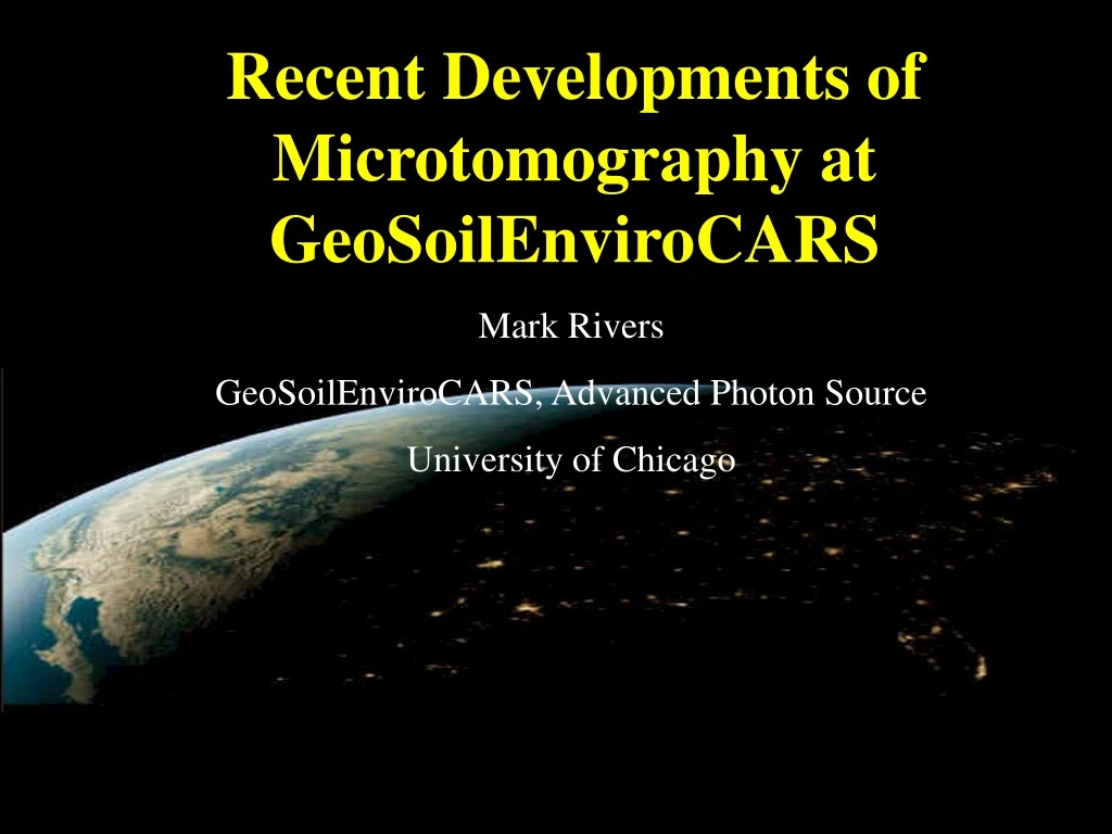
1. Recent Developments of Microtomography at GeoSoilEnviroCARS Mark Rivers GeoSoilEnviroCARS, Advanced Photon Source University of Chicago

2. Outline of Talk • Tomography at extreme conditions • High pressure • High speed • (High temperature, low temperature) • Recent technical developments • Reconstruction speeds • Visible light optics • Ring artifact reduction • Rotation stage imprecision

3. Microscope objective Sample Scintillator CCD camera X-rays X-rays Visible light Rotation stage Absorption Tomography Setup13-BM-D station at APS • X-ray Source • Parallel monochromatic x-rays, 8-65 keV • APS bending magnet source, 20 keV critical energy • 1-50mm field of view in horizontal, up to 6 mm in vertical • Imaging System • YAG or CdWO4 single crystal scintillator • 5X to 20X microscope objectives, or macro lens • 1300 x 1030 pixel, 12-bit CCD camera • Data collection • Rotate sample 180 degrees, acquire images every 0.25 degrees • Data collection time: 10 minutes • Reconstruction time: 5 minutes

4. 32.5 keV, below I and Cs K absorption edges 33.2 keV, above I and below Cs K absorption edges 36.0 keV, above I and Cs K absorption edges 36.0 - 33.2, showing distribution of Cs in the aqueous phase 33.2 - 32.5 keV, showing distribution of I in the organic phase Differential Absorption TomographyClint Willson (Louisiana State University) 8mm diameter sand column with aqueous phase containing Cs and organic phase containing I.

5. 250 T press frame Die set Harmonic Drive Transport Rails Hydraulic ram High-P tomography: Instrumentation Thrust bearings Max. load 50 tons

6. High pressure tomography: setupCurrent pressure maxium=10GPa (100 kbar)Goal: 20 GPa (200 kbar) Top view Fe – S alloy CCD detector Al2O3 Microscope objective Phosphor (YAG) Monochromator Mirror Sample Incident X-rays (white) Rotation Drickamer Visible light Transmitted X-rays Monochromatic beam

7. Anvil Fe0.9S0.1 BE BN Anvil 803 µm vitreous forsterite sphere 0 tons Gaudio, Lesher, Wang, Nishiyama

9. High-Speed Radiography ofGranular Particle JetsJohn Royer,University of Chicago Physics Dept. Sphere falling into a granular particle (e.g. sand) bed produces a jet These images are above the surface, done with visible light 1 atmosphere Reduced pressure

10. Want to understand what is happening below the surface Used “pink” x-ray beam, high speed radiography 100 msec exposure time, 5000 frames/sec

11. Processing Times • Data processing is done in 2 steps using IDL graphical user-interface • Pre-processing: dark current and flat field normalization, zinger removal • Sinogram calculation and reconstuction • Reconstruction is done with Gridrec FFT-based C code from Brookhaven. • No measureable difference from FBP, but >15X faster. • Recently changed from Intel MKL or Numerical Recipes FFT to the FFTW package. 3-4 times faster. • Upgraded to dual 3.4 GHz Intel, 8GB RAM, 64-bit Linux, 64-bit IDL, • FFTW is built single-threaded, second CPU is idle for other tasks

12. Optics Improvements • We have been using Mitutoyu long working distance microscope objectives with various tube lens to achieve the desired fields of view. This often involved shorter tube lens than the nominal 200mm tube length. • Recently purchased a Nikon macro lens. This lens allows various fields of view, depending on how the lens is focus, and what extension tubes if any are used. • We have now compared images collected with very similar pixel sizes using the Mitutoyu lenses and the Nikon lens. It is clear that at least at fields of view > 6mm the Nikon lens is significantly sharper. Sand and fluid, 33.269 keV, Z slice Mitutoyu 5X, 17.5mm tube, 11.1 micron pixels Nikon lens, PK-11A extender, 11.2 micron pixels

13. Another example of improvement in optics Meteorite, 38 keV, Y slices Mitutoyu 5X, 17.5mm tube, 11.1 micron pixels Nikon lens, PK-11A extender, 11.2 micron pixels

14. Ring Artifact Reduction - Algorithm • Compute average of all rows in sinogram • This should be a smooth function with little high-frequency content • Compute a smoothed version of the average with user-selectable smoothing width. • Unsmoothed version minus smoothed version is the correction factor for that pixel • Subtract the correction from that pixel in every projection

15. Ring Artifact Reduction - Sinograms Sinogram before correction Sinogram after correction with 21-point smoothing

16. Ring Artifact Reduction - Reconstructions No correction 9-point smooth 21-point smooth

17. Ring Artifacts – A Puzzle • We often found ring artifacts even after applying the preceeding algorithm Ring artifact suppression=Off Ring artifact suppression=9 point

18. Ring Artifacts – the Flat Field Problem • We finally realized that these rings were arising from the flat fields • This image was reconstructed simply assuming a constant flat field of 4000 counts! Many fewer rings! Ring artifact suppression=Off Ring artifact suppression=9 point

19. Ring Artifacts – Major Improvement • We were previously interpolating the flat fields with time to best estimate the flat field when each projection was taken • This introduced 2 serious problems: • Noise in the flat field images resulted in anomalous pixels (rings) in many projections • The resulting “rings” were only partial rings, not semi-circles, because each noisy pixel was only used over an angular range of 12-25 degrees. • This greatly reduced the efficacy of the ring artifact reduction algorithm • Solution was easy: • Average all the flat fields, rather than interpolating them • Better solution would be to collect many flat fields periodically, then average and interpolate

20. Ring Artifacts – Using Flat Field Averaging Ring artifact suppression=Off Ring artifact suppression=9 point

21. Ring Artifacts – Another Example New default, flat field averaging, 9-point smooth for reduction Old default, flat field interpolation, 9-point smooth for reduction

22. Rotation Stage Imperfections • When doing high-resolution tomography we have seen small horizontal shifts in the sinogram at some angles. • This is due to mechanical imprecision (eccentricity, wobble) in the stage Sinogram with small horizontal shifts at some angles Enlargement of lower right, showing shifts more prominently

23. Rotation Stage Corrections • Developed an algorithm to correct these shifts using only the sinogram data itself. • The center of gravity of each row of the sinogram (average of horizontal distance X –log(I/I0)) itself must describe a sine wave • Fit the sine wave to the center of gravity for the sinogram of each slice. Measure the deviation from the best-fit sine wave • Some of that deviation is noise, some is systematic error due to mechanical shifts in the stage • The mechanical shifts should be the same for every slice, thus we can reduce noise by averaging over all slices • Must reject slices with no meaningful center-of-gravity, i.e. slices with just air or with complete absorption

24. Rotation Stage Corrections

25. Rotation Stage Corrections - Sinograms Enlargement of sinogram before correction Enlargement of sinogram after correction

26. Rotation Stage Corrections - Reconstructions Reconstruction after correction Reconstruction before correction

27. Rotation Stage Corrections - Reconstructions Enlargement of reconstruction before correction Enlargement of reconstruction after correction

28. Rotation Stage Corrections – Laser Autocollimator Measurements • Used Newport LAE500 laser autocollimator with high-precision reflective ball to measure rotation motion in horizontal and vertical • Mounted ball near center of rotation, fit sine-wave for expected motion • Deviations from sine-wave are errors in horizontal and vertical

29. Laser Autocollimator MeasurementsOld Newport URM-80 Stage

30. Laser Autocollimator MeasurementsNew Newport URM-80 Stage

31. Rotation Stage Corrections – Conclusions • Software can automatically correct for rotation axis imperfection • Our stage was particularly bad at ~3-4 microns, but as resolution is pushed to sub-micron tomography there will be a real benefit from these corrections • Laser autocollimator is very useful for evaluating stages