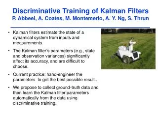
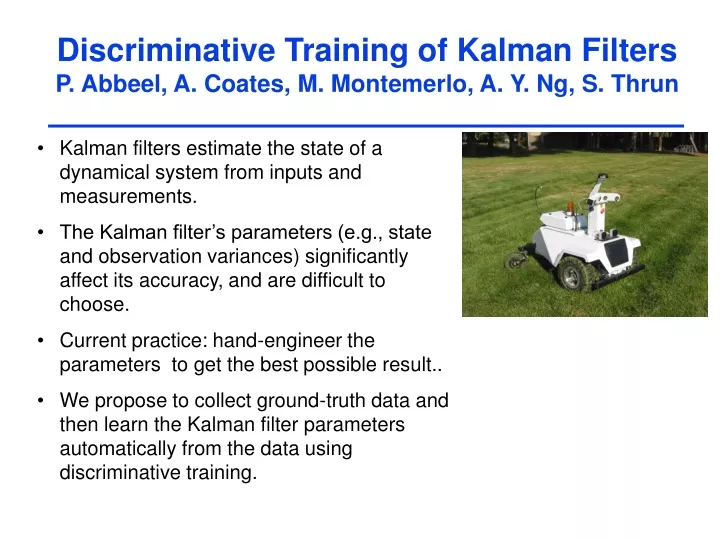
Discriminative Training of Kalman Filters P. Abbeel, A. Coates, M. Montemerlo, A. Y. Ng, S. Thrun

1. Discriminative Training of Kalman FiltersP. Abbeel, A. Coates, M. Montemerlo, A. Y. Ng, S. Thrun • Kalman filters estimate the state of a dynamical system from inputs and measurements. • The Kalman filter’s parameters (e.g., state and observation variances) significantly affect its accuracy, and are difficult to choose. • Current practice: hand-engineer the parameters to get the best possible result.. • We propose to collect ground-truth data and then learn the Kalman filter parameters automatically from the data using discriminative training.

2. Discriminative Training of Kalman FiltersP. Abbeel, A. Coates, M. Montemerlo, A. Y. Ng, S. Thrun Ground truth Hand-engineered Learned

3. Discriminative Training of Kalman Filters Pieter Abbeel, Adam Coates, Mike Montermerlo, Andrew Y. Ng, Sebastian Thrun Stanford University

4. Motivation • Extended Kalman filters (EKFs) estimate the state of a dynamical system from inputs and measurements. • For fixed inputs and measurements, the estimated state sequence depends on: • Next-state function. • Measurement function. • Noise model.

5. Motivation (2) • Noise terms typically result from a number of different effects: • Mis-modeled system dynamics and measurement dynamics. • The existence of hidden state in the environment not modeled by the EKF. • The discretization of time. • The algorithmic approximations of the EKF itself, such as the Taylor approximation commonly used for linearization. • In Kalman filters noise is assumed independent over time, in practice noise is highly correlated.

6. Motivation (3) • Common practice: careful hand-engineering of the Kalman filter’s parameters to optimize its performance, which can be very time consuming. • Proposed solution: automatic learning of the Kalman filter’s parameters from data where (part of) the state-sequence is observed (or very accurately measured). • In this work: we focus on learning the state and measurement variances, although the principles are more generally applicable.

7. Example • Problem: estimate the variance of a GPS unit used to estimate the fixed position x of a robot. • Standard model: • xmeasured = xtrue +  • » N(0,2) (Gaussian with mean 0, variance 2) • Assuming the noise is independent over time, we have after n measurements variance = 2/n. • However if the noise is perfectly correlated, the true variance is 2 >> 2/n. • Practical implication: wrongly assuming independence leads to overconfidence in the GPS sensor. This matters not only for the variance, but also for the state estimate when information from multiple sensors is combined.

8. Extended Kalman filter • State transition equation: • xt = f(xt-1,ut) +  • » N(0, R) (Gaussian with mean zero, covariance R) • Measurement equation: • zt = g(xt) +  • » N(0,Q) (Gaussian with mean zero, covariance Q) • The extended Kalman filter linearizes the non-linear function f, g through their Taylor approximation: • f(xt-1,ut) ¼f(t-1,ut) + Ft(xt-1-t-1) • g(xt) ¼g(t) + Gt(xt - t) Here Ft and Gt are Jacobian matrices of f and g respectively, taken at the filter estimate .

9. Extended Kalman Filter (2) • For linear systems, the (standard) Kalman filter produces exact updates of expected state and covariance. The extended Kalman filter applies the same updates to the linearized system. • Prediction update step: • Place holder • Place holder • Measurement update step: • Place holder • Place holder • Place holder

10. Discriminative training • Let y be a subset of the state variables x for which we obtain ground-truth data. E.g., the positions obtained with a very high-end GPS receiver that is not part of the robot system when deployed. • We use h(.) to denote the projection from x to y: y = h(x). • Discriminative training: • Given (u1:T, z1:T, y1:T). • Find the filter parameters that predict y1:T most accurately. [Note: it is actually sufficient that y is a highly accurate estimate of x. See the paper for details.]

11. Three discriminative training criteria • Minimizing the residual prediction error: • Maximizing the prediction likelihood: • Maximizing the measurement likelihood: (The last criterion does not require access to y1:T.)

12. Evaluating the training criteria • The extended Kalman filter computes p(xt|z1:t,u1:t) = N(t, t) for all times t2 {1 … T}. • Residual prediction error and prediction likelihood can be evaluated directly from the filter’s output. • Measurement likelihood:

13. Robot testbed

14. The robot’s state, inputs and measurements • State: • x,y : position coordinates. • : heading. • v : velocity. • b : gyro bias. • Control inputs: • r : rotational velocity. • a : forward acceleration. • Measurements: • Optical wheel encoders measure v. • A (cheap) GPS unit measures x,y (1Hz, 3m accuracy). • A magnetic compass measures .

15. System Equations

16. Experimental setup • We collected two data sets (100 seconds each) by driving the vehicle around on a grass field. One data set is used to discriminatively learn the parameters, the other data set is used to evaluate the performance of the different algorithms. • A Novatel RT2 differential GPS unit (10Hz, 2cm accuracy) was used to obtain ground truth position data. Note the hardware on which our algorithms are evaluated do not have the more accurate GPS.

17. Experimental results (1) • Evaluation metrics: • RMS error (on position): • Prediction log-loss (on position):

18. Ground truth CMU hand-engineered Learned minimizing residual prediction error Experimental results (2) Zoomed in on this area on next figure.

19. Ground truth CMU hand-engineered Learned minimizing residual prediction error Experimental results (3)

20. Ground truth CMU hand-engineered Learned minimizing residual prediction error Learned maximizing prediction likelihood Learned maximizing measurement likelihood Experimental Results (4) Zoomed in on this area on next figure. x (cheap) GPS

21. Ground truth CMU hand-engineered Learned minimizing residual prediction error Learned maximizing prediction likelihood Learned maximizing measurement likelihood Experimental Results (5) x (cheap) GPS

22. Related Work • Conditional Random Fields (J. Lafferty, A. McCallum, F. Pereira, 2001). The optimization criterion (translated to our setting) is: • Issues for our setting: • The criterion does not use filter estimates. (It uses smoother estimates instead.) • The criterion assumes the state is fully observed.

23. Discussion and conclusion • In practice Kalman filters often require time-consuming hand-engineering of the noise parameters to get optimal performance. • We presented a family of algorithms that use a discriminative criterion to learn the noise parameters automatically from data. • Advantages: • Eliminates hand-engineering step. • More accurate state estimation than even a carefully hand-engineered filter.

24. Discriminative

25. Training of

26. Kalman Filters

27. Pieter Abbeel, Adam Coates, Mike Montemerlo, Andrew Y. Ng and Sebastian Thrun Stanford University

28. Pieter Abbeel, Adam Coates, Mike Montemerlo, Andrew Y. Ng and Sebastian Thrun Stanford University

29. Robot testbed