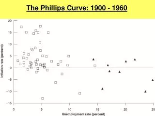
The Phillips Curve: 1900 - 1960
120 likes | 380 Vues
The Phillips Curve: 1900 - 1960. The Early Incarnation, Circa 1960. 1970s Stagflation : Why did the Phillips curve vanish? Is there no inflation – unemployment tradeoff?. Inflation & Expectations: Natural rate hypothesis 1970-1998: t – t-1 = 6.5% – 1.0u t = -1 ( u t - 6.5%)

The Phillips Curve: 1900 - 1960
E N D
Presentation Transcript
1970s Stagflation: Why did the Phillips curve vanish?Is there no inflation – unemployment tradeoff?
Inflation & Expectations: Natural rate hypothesis • 1970-1998: t – t-1 = 6.5% – 1.0ut = -1 (ut - 6.5%) • Acceleration hypothesis: keep ut < uN rises year after year • But late 1990s – 2007: “low” unemployment without much inflation Expectations augmented Phillips Curve shifts
The Phillips Curve – Differences in the “Natural Rate” Across Countries Europe in the 1990s
Expectations Augmented Phillips Curve • From our wage setting – price setting model: • Wt = Pte F(ut,z) and Pt = (1+µ) Wt • Let F(ut,z) = 1 - ut + z • Then Pt = Pte (1 + µ) F(ut,z) • Pt = Pte (1 + µ) (1 - ut + z) • We can then derive • t = te + (µ+z) - ut • where • t = the inflation rate • te = expected inflation rate • = Sensitivity of wages to the unemployment rate • When t = te(medium-run equilibrium) • u = (µ+z)/ = “natural rate” of unemployment
Determinants of “Natural” Rate of Unemployment • µ = Markup over unit labor cost • Degree of monopoly (elasticities of demand) • Other input costs: energy/imports/… • Z = Structural factors • Unemployment benefits • Labor militancy • International competition • Government stance: Air Traffic Controllers Strike • Implicit contracts: Japanese life-long jobs • Structural change • Hysteresis: History matters
Monetary Policy Macro-stabilityOutput, Unemployment, & Inflation Tools for Disinflation • Modified Phillips Curve: unemployment and the change in inflation • Okun’s Law: output growth and the change in unemployment • Aggregate Demand: Money, output, and prices Money growth, Output growth, Inflation
Okun’s Law: The Equation ut - ut-1 = - 0.4 (gyt - 3%) • gyt must be at least 3% to keep unemployment from rising • WHY? • Labor force growth • Increases in labor productivity • Why is the coefficient only 0.4? • Firms need a minimum number of workers • Firms hoard labor • Changes in labor force participation • When economy tanks, workers drop out of the laborforce • u doesn’t rise as much as it otherwise would • Okun’s Law Coefficients Across Countries • Country 1960-1980 1981-1998 • United States 0.39 0.42 United Kingdom 0.15 0.51 Germany* 0.20 0.32 Japan 0.10 0.20
Okun’s Law : how growth in excess of normal growth impacts the unemployment rate : normal growth rate In general, the relation between changes in unem-ployment and output growth is: