Chapter 2:Inventory Management and Risk Pooling
Chapter 2:Inventory Management and Risk Pooling. CASE: Steel Works. Background of case and intent Overview of business What does data tell you about Specialty? How much inventory might you expect? What opportunities are there for Custom? Wrap up. Background & Intent.

Chapter 2:Inventory Management and Risk Pooling
E N D
Presentation Transcript
CASE: Steel Works • Background of case and intent • Overview of business • What does data tell you about Specialty? • How much inventory might you expect? • What opportunities are there for Custom? • Wrap up
Background & Intent • Abstraction from summer consulting job • Intent is to examine a realistic, but simplified inventory context and perform a diagnosis of problem – poor service and too much inventory
Custom Products • Rapid growth, 1/3 of total sales ($133 MM) • One customer per product • Very high margins • High service level • 3 plants, co-located with R&D center • Each product produced at a single plant
Specialty Products • Rapid growth, 2/3 of total sales ($267 MM) • 6 product families • 3 plants, each producing 2 product families • 130 customers, 120 products • Few big customers • Highly volatile demand • High service level
Consultant Recommendation • Drop low volume products • Improve forecasts • Consolidate warehouses
What Does Data Tell You? • Durabend R12: • One customer accounts for 97% of demand • 7 products: • High volume (2) is not very volatile • Low volume (5) is very volatile
How Much Inventory Should You Expect? • Assume base stock model with periodic review • Review period = r = ? • Lead time = L = ?
Assumes r = 1; L=0.25; and z = 1.8 Cycle stock = r m/2 Safety stock = z sr+L
What Are the Opportunities at Custom? • Combine production and inventory for common items, e. g. DF R23 • Produce monthly: reduce setups by half and pool safety stocks • Produce twice a month: same number of setups but cut cycle stock and review period in half
Wrap Up • Realistic diagnostic exercise • In real life: not as clean, more data and more considerations • Yet simple models and principles can provide valuable guidance
2.1 IntroductionWhy Is Inventory Important? Distribution and inventory (logistics) costs are quite substantial Total U.S. Manufacturing Inventories ($m): • 1992-01-31: $m 808,773 • 1996-08-31: $m 1,000,774 • 2006-05-31: $m 1,324,108 Inventory-Sales Ratio (U.S. Manufacturers): • 1992-01-01: 1.56 • 2006-05-01: 1.25
Why Is Inventory Important? • GM’s production and distribution network • 20,000 supplier plants • 133 parts plants • 31 assembly plants • 11,000 dealers • Freight transportation costs: $4.1 billion (60% for material shipments) • GM inventory valued at $7.4 billion (70%WIP; Rest Finished Vehicles) • Decision tool to reduce: • combined corporate cost of inventory and transportation. • 26% annual cost reduction by adjusting: • Shipment sizes (inventory policy) • Routes (transportation strategy)
Why Is Inventory Required? • Uncertainty in customer demand • Shorter product lifecycles • More competing products • Uncertainty in supplies • Quality/Quantity/Costs/Delivery Times • Delivery lead times • Incentives for larger shipments
Holding the right amount at the right time is difficult! • Dell Computer’s was sharply off in its forecast of demand, resulting in inventory write-downs • 1993 stock plunge • Liz Claiborne’s higher-than-anticipated excess inventories • 1993 unexpected earnings decline, • IBM’s ineffective inventory management • 1994 shortages in the ThinkPad line • Cisco’s declining sales • 2001 $ 2.25B excess inventory charge
Inventory Management-Demand Forecasts • Uncertain demand makes demand forecast critical for inventory related decisions: • What to order? • When to order? • How much is the optimal order quantity? • Approach includes a set of techniques • INVENTORY POLICY!!
Supply Chain Factors in Inventory Policy • Estimation of customer demand • Replenishment lead time • The number of different products being considered • The length of the planning horizon • Costs • Order cost: • Product cost • Transportation cost • Inventory holding cost, or inventory carrying cost: • State taxes, property taxes, and insurance on inventories • Maintenance costs • Obsolescence cost • Opportunity costs • Service level requirements
2.2 Single Stage Inventory Control • Single supply chain stage • Variety of techniques • Economic Lot Size Model • Demand Uncertainty • Single Period Models • Initial Inventory • Multiple Order Opportunities • Continuous Review Policy • Variable Lead Times • Periodic Review Policy • Service Level Optimization
2.2.1. Economic Lot Size Model FIGURE 2-3: Inventory level as a function of time
Assumptions • D items per day: Constant demand rate • Q items per order: Order quantities are fixed, i.e., each time the warehouse places an order, it is for Q items. • K, fixed setup cost, incurred every time the warehouse places an order. • h, inventory carrying cost accrued per unit held in inventory per day that the unit is held (also known as, holding cost) • Lead time = 0 (the time that elapses between the placement of an order and its receipt) • Initial inventory = 0 • Planning horizon is long (infinite).
Deriving EOQ • Total cost at every cycle: • Average inventory holding cost in a cycle: Q/2 • Cycle timeT =Q/D • Average total cost per unit time:
EOQ: Costs FIGURE 2-4: Economic lot size model: total cost per unit time
Sensitivity Analysis Total inventory cost relatively insensitive to order quantities Actual order quantity: Q Q is a multiple b of the optimal order quantity Q*. For a given b, the quantity ordered is Q = bQ*
2.2.2. Demand Uncertainty • The forecast is always wrong • It is difficult to match supply and demand • The longer the forecast horizon, the worse the forecast • It is even more difficult if one needs to predict customer demand for a long period of time • Aggregate forecasts are more accurate. • More difficult to predict customer demand for individual SKUs • Much easier to predict demand across all SKUs within one product family
2.2.3. Single Period Models Short lifecycle products • One ordering opportunity only • Order quantity to be decided before demand occurs • Order Quantity > Demand => Dispose excess inventory • Order Quantity < Demand => Lose sales/profits
Single Period Models • Using historical data • identify a variety of demand scenarios • determine probability each of these scenarios will occur • Given a specific inventory policy • determine the profit associated with a particular scenario • given a specific order quantity • weight each scenario’s profit by the likelihood that it will occur • determine the average, or expected, profit for a particular ordering quantity. • Order the quantity that maximizes the average profit.
Single Period Model Example FIGURE 2-5: Probabilistic forecast
Additional Information • Fixed production cost: $100,000 • Variable production cost per unit: $80. • During the summer season, selling price: $125 per unit. • Salvage value: Any swimsuit not sold during the summer season is sold to a discount store for $20.
Two Scenarios • Manufacturer produces 10,000 units while demand ends at 12,000 swimsuits Profit = 125(10,000) - 80(10,000) - 100,000 = $350,000 • Manufacturer produces 10,000 units while demand ends at 8,000 swimsuits Profit = 125(8,000) + 20(2,000) - 80(10,000) - 100,000 = $140,000
Probability of Profitability Scenarios with Production = 10,000 Units • Probability of demand being 8000 units = 11% • Probability of profit of $140,000 = 11% • Probability of demand being 12000 units = 27% • Probability of profit of $140,000 = 27% • Total profit = Weighted average of profit scenarios
Order Quantity that Maximizes Expected Profit FIGURE 2-6: Average profit as a function of production quantity
Relationship Between Optimal Quantity and Average Demand • Compare marginal profit of selling an additional unit and marginal cost of not selling an additional unit • Marginal profit/unit = Selling Price - Variable Ordering (or, Production) Cost • Marginal cost/unit = Variable Ordering (or, Production) Cost - Salvage Value • If Marginal Profit > Marginal Cost => Optimal Quantity > Average Demand • If Marginal Profit < Marginal Cost => Optimal Quantity < Average Demand
For the Swimsuit Example • Average demand = 13,000 units. • Optimal production quantity = 12,000 units. • Marginal profit = $45 • Marginal cost = $60. • Thus, Marginal Cost > Marginal Profit => optimal production quantity < average demand.
Risk-Reward Tradeoffs • Optimal production quantity maximizes average profit is about 12,000 • Producing 9,000 units or producing 16,000 units will lead to about the same average profit of $294,000. • If we had to choose between producing 9,000 units and 16,000 units, which one should we choose?
Risk-Reward Tradeoffs FIGURE 2-7: A frequency histogram of profit
Risk-Reward Tradeoffs • Production Quantity = 9000 units • Profit is: • either $200,000 with probability of about 11 % • or $305,000 with probability of about 89 % • Production quantity = 16,000 units. • Distribution of profit is not symmetrical. • Losses of $220,000 about 11% of the time • Profits of at least $410,000 about 50% of the time • With the same average profit, increasing the production quantity: • Increases the possible risk • Increases the possible reward
Observations • The optimal order quantity is not necessarily equal to forecast, or average, demand. • As the order quantity increases, average profit typically increases until the production quantity reaches a certain value, after which the average profit starts decreasing. • Risk/Reward trade-off: As we increase the production quantity, both risk and reward increases.
2.2.4. What If the Manufacturer Has an Initial Inventory? • Trade-off between: • Using on-hand inventory to meet demand and avoid paying fixed production cost: need sufficient inventory stock • Paying the fixed cost of production and not have as much inventory
Initial Inventory Solution FIGURE 2-8: Profit and the impact of initial inventory
Manufacturer Initial Inventory = 5,000 • If nothing is produced, average profit = 225,000 (from the figure) + 5,000 x 80 = 625,000 • If the manufacturer decides to produce • Production should increase inventory from 5,000 units to 12,000 units. • Average profit = 371,000 (from the figure) + 5,000 • 80 = 771,000
Manufacturer Initial Inventory = 10,000 • No need to produce anything • average profit > profit achieved if we produce to increase inventory to 12,000 units • If we produce, the most we can make on average is a profit of $375,000. • Same average profit with initial inventory of 8,500 units and not producing anything. • If initial inventory < 8,500 units => produce to raise the inventory level to 12,000 units. • If initial inventory is at least 8,500 units, we should not produce anything (s, S) policy or (min, max) policy
2.2.5. Multiple Order Opportunities REASONS • To balance annual inventory holding costs and annual fixed order costs. • To satisfy demand occurring during lead time. • To protect against uncertainty in demand. TWO POLICIES • Continuous review policy • inventory is reviewed continuously • an order is placed when the inventory reaches a particular level or reorder point. • inventory can be continuously reviewed (computerized inventory systems are used) • Periodic review policy • inventory is reviewed at regular intervals • appropriate quantity is ordered after each review. • it is impossible or inconvenient to frequently review inventory and place orders if necessary.
2.2.6. Continuous Review Policy • Daily demand is random and follows a normal distribution. • Every time the distributor places an order from the manufacturer, the distributor pays a fixed cost, K, plus an amount proportional to the quantity ordered. • Inventory holding cost is charged per item per unit time. • Inventory level is continuously reviewed, and if an order is placed, the order arrives after the appropriate lead time. • If a customer order arrives when there is no inventory on hand to fill the order (i.e., when the distributor is stocked out), the order is lost. • The distributor specifies a required service level.
Continuous Review Policy • AVG = Average daily demand faced by the distributor • STD = Standard deviation of daily demand faced by the distributor • L = Replenishment lead time from the supplier to the • distributor in days • h = Cost of holding one unit of the product for one day at the distributor • α = service level. This implies that the probability of stocking out is 1 - α
Continuous Review Policy • (Q,R) policy – whenever inventory level falls to a reorder level R, place an order for Q units • What is the value of R?
Continuous Review Policy • Average demand during lead time: L x AVG • Safety stock: • Reorder Level, R: • Order Quantity, Q:
Service Level & Safety Factor, z z is chosen from statistical tables to ensure that the probability of stockouts during lead time is exactly 1 - α
Inventory Level Over Time FIGURE 2-9: Inventory level as a function of time in a (Q,R) policy Inventory level before receiving an order = Inventory level after receiving an order = Average Inventory =
Continuous Review Policy Example • A distributor of TV sets that orders from a manufacturer and sells to retailers • Fixed ordering cost = $4,500 • Cost of a TV set to the distributor = $250 • Annual inventory holding cost = 18% of product cost • Replenishment lead time = 2 weeks • Expected service level = 97%