HDRI Capture and Response Curve Recovery Utilizing Multiple Exposures

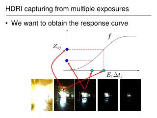
HDRI capturing from multiple exposures • We want to obtain the response curve

HDRI capturing from multiple exposures Image series • 1 • 1 • 1 • 1 • 1 • 2 • 2 • 2 • 2 • 2 • 3 • 3 • 3 • 3 • 3 Dt =2 sec Dt =1 sec Dt =1/2 sec Dt =1/4 sec Dt =1/8 sec

Idea behind the math

Math for recovering response curve

Recovering response curve • The solution can be only up to a scale, add a constraint • Add a hat weighting function

How to optimize? • Set partial derivatives zero

: : Sparse linear system n 256 g(0) n×p : g(255) lnE1 lnEn 1 254 Ax=b

Questions • Will g(127)=0 always be satisfied? Why and why not? • How to find the least-square solution for an over-determined system?

The are often mutually incompatible. We instead find x to minimize the norm of the residual vector . If there are multiple solutions, we prefer the one with the minimal length . Least-square solution for a linear system

pseudo inverse Least-square solution for a linear system If we perform SVD on A and rewrite it as then is the least-square solution.

Libraries for SVD • Matlab • GSL • Boost • LAPACK (recommended) • ATLAS

Matlab code

Matlab code function [g,lE]=gsolve(Z,B,l,w) n = 256; A = zeros(size(Z,1)*size(Z,2)+n+1,n+size(Z,1)); b = zeros(size(A,1),1); k = 1; %% Include the data-fitting equations for i=1:size(Z,1) for j=1:size(Z,2) wij = w(Z(i,j)+1); A(k,Z(i,j)+1) = wij; A(k,n+i) = -wij; b(k,1) = wij * B(i,j); k=k+1; end end A(k,129) = 1; %% Fix the curve by setting its middle value to 0 k=k+1; for i=1:n-2 %% Include the smoothness equations A(k,i)=l*w(i+1); A(k,i+1)=-2*l*w(i+1); A(k,i+2)=l*w(i+1); k=k+1; end x = A\b; %% Solve the system using SVD g = x(1:n); lE = x(n+1:size(x,1));

Recovered response function

Recovering response curve • We want If P=11, N~25 (typically 50 is used) • We prefer that selected pixels are well distributed and sampled from constant regions. They picked points by hand. • It is an overdetermined system of linear equations and can be solved using SVD

Constructing HDR radiance map combine pixels to reduce noise and obtain a more reliable estimation

Varying shutter speeds

Reconstructed radiance map

What is this for? • Human perception • Vision/graphics applications

Radiance format (.pic, .hdr, .rad) 32 bits/pixel Red Green Blue Exponent (145, 215, 87, 103) = (145, 215, 87) * 2^(103-128) = (0.00000432, 0.00000641, 0.00000259) (145, 215, 87, 149) = (145, 215, 87) * 2^(149-128) = (1190000, 1760000, 713000) Ward, Greg. "Real Pixels," in Graphics Gems IV, edited by James Arvo, Academic Press, 1994

Demo http://www.hdrsoft.com/examples.html

Image alignment

Median Threshold Bitmap (MTB) alignment • Consider only integral translations. It is enough empirically. • The inputs are N grayscale images. (You can either use the green channel or convert into grayscale by Y=(54R+183G+19B)/256) • MTB is a binary image formed by thresholding the input image using the median of intensities.

Search for the optimal offset • Try all possible offsets. • Gradient descent • Multiscale technique • log(max_offset) levels • Try 9 possibilities for the top level • Scale by 2 when passing down; try its 9 neighbors

ignore pixels that are close to the threshold exclusion bitmap Threshold noise

Results Success rate = 84%. 10% failure due to rotation. 3% for excessive motion and 3% for too much high-frequency content.

Equipment We provide 3 sets: Contact TA for checkout.

HDRI Capture and Response Curve Recovery Utilizing Multiple Exposures