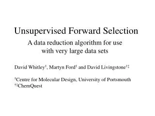
Unsupervised Forward Selection

1. Unsupervised Forward Selection A data reduction algorithm for use with very large data sets David Whitley†, Martyn Ford† and David Livingstone†‡ †Centre for Molecular Design, University of Portsmouth †‡ChemQuest

2. Outline • Variable selection issues • Pre-processing strategy • Dealing with multicollinearity • Unsupervised forward selection • Model selection strategy • Applications

3. Variable Selection Issues • Relevance • statistically significant correlation with response • non-small variance • Redundancy • linear dependence • some variables have no unique information • Multicollinearity • near linear dependence • some variables have little unique information

4. Pre-processing Strategy • Identify variables with a significant correlation with the response • Remove variables with small variance • Remove variables with no unique information • Identify a set of variables on which to construct a model

5. Effect of Multicollinearity Build regression models of the form where and x1 - x4 , y, zi and ei are random N(0,1) Increasing  reduces the collinearity between x5 and x1

6. Effect of Multicollinearity Q2 

7. Dealing with Multicollinearity • Examine pair-wise correlations between variables, and remove one from each pair with high correlation • Corchop (Livingstone & Rahr, 1989) aims to remove the smallest number of variables while breaking the largest number of pair-wise collinearities

8. Unsupervised Forward Selection • Select the first two variables with the smallest pair-wise correlation coefficient • Reject variables whose pair-wise correlation coefficient with the selected columns exceeds rsqmax • Select the next variable to have the smallest squared multiple correlation coefficient with those previously selected • Reject variables with squared multiple correlation coefficients greater than rsqmax • Repeat 3 - 4 until all variables are selected or rejected

9. Continuum Regression • A regression procedure with the generalized criterion function • Varying the continuous parameter 0   1.5 adjusts the balance between the covariance of the response with the descriptors and the variance of the descriptors, so that •  = 0 is equivalent to ordinary least squares •  = 0.5 is equivalent to partial least squares •  = 1.0 is equivalent to principal components regression

10. Model Selection Strategy • For  = 0.0, 0.1, …, 1.5 build a CR model for the set of variables selected by UFS with rsqmax = 0.1, 0.2, …, 0.9, 0.99 • Select the model with rsqmax and  maximizing Q2 (leave-one-out cross-validated R2) • Apply n-fold cross-validation to check predictive ability • Apply a randomization test (1000 permutations of the response scores) to guard against chance correlation

11. Pyrethroid Data Set • 70 physicochemical descriptors to predict killing activity (KA) of 19 pyrethroid insecticides • Only 6 descriptors are correlated with KA at the 5% level • Optimal models • 4-variable, 2-component model with R2 = 0.775, Q2 = 0.773 obtained when rsqmax = 0.7,  = 1.2 • 3-variable, 1-component model with R2 = 0.81, Q2 = 0.76 obtained when rsqmax = 0.6,  = 0.2

12. Optimal Model I • Standard errors are bootstrap estimates based on 5000 bootstraps • Randomization test tail probabilities below 0.0003 for fit and 0.0071 for prediction

13. Optimal Model II • Standard errors are bootstrap estimates based on 5000 bootstraps • Randomization test tail probabilities below 0.0001 for fit and 0.0052 for prediction

14. N-Fold Cross-Validation 4 variable model 3 variable model

15. Feature Recognition • Important explanatory variables may not be selected for inclusion in the model • force some variables in, then continue UFS algorithm • The component loadings for the original variables can be examined to identify variables highly correlated with the components in the model

16. Loadings for the 1-component pyrethroid model with tail probability < 0.01

17. Steroid Data Set • 21 steroid compounds from SYBYL CoMFA tutorial to model binding affinity to human TBG • Initial data set has 1248 variables with values below 30 kcal/mol • Removed 858 variables not significantly correlated with response (5% level) • Removed 367 variables with variance below 1.0 kcal/mol • Leaving 23 variables to be processed by UFS/CR

18. Optimal models • UFS/CR produces a 3-variable, 1-component model with R2 = 0.85, Q2 = 0.83 at rsqmax = 0.3,  = 0.3 • CoMFA tutorial produces a 5-component model with R2 = 0.98, Q2 = 0.6

19. N-Fold Cross-Validation CoMFA tutorial model UFS/CR model

20. Putative Pharmacophore

21. Selwood Data Set • 53 descriptors to predict biological activity of 31 antifilarial antimycin analogues • 12 descriptors are correlated with the response variable at the 5% level • Optimal models • 2-variable, 1-component model with R2 = 0.42, Q2 = 0.41 obtained when rsqmax = 0.1,  = 1.0 • 12-variable, 1-component model with R2 = 0.85, Q2 = 0.5 obtained when rsqmax = 0.99,  = 0.0 (omitting compound M6)

22. N-Fold Cross-Validation 2-variable model 12-variable model

23. Summary • Multicollinearity is a potential cause of poor predictive power in regression. • The UFS algorithm eliminates redundancy and reduces multicollinearity, thus improving the chances of obtaining robust, low-dimensional regression models. • Chance correlation can be addressed by eliminating variables that are uncorrelated with the response.

24. Summary • UFS can be used to adjust the balance between reducing multicollinearity and including relevant information. • Case studies show that leave-one-out cross-validation should be supplemented by n-fold cross-validation, in order to obtain accurate and precise estimates of predictive ability (Q2).

25. Acknowledgements BBSRC Cooperation with Industry Project: Improved Mathematical Methods for Drug Design • Astra Zeneca • GlaxoSmithKline • MSI • Unilever

26. Reference D. C. Whitley, M.G. Ford and D. J. Livingstone Unsupervised forward selection: a method for eliminating redundant variables. J. Chem. Inf. Comp. Sci., 2000, 40, 1160-1168. UFS software available from: http://www.cmd.port.ac.uk CR is a component of Paragon (available summer 2001)