5. Distributed Database Design
5. Distributed Database Design. Chapter 3 Distributed Database Design. Outline. Introduction Fragmentation (片段划分) Horizontal fragmentation (水平划分) Derived horizontal fragmentation (导出式水平划分) Vertical fragmentation (垂直划分) Allocation (片段分配). Outline. Introduction Fragmentation (片段划分)

5. Distributed Database Design
E N D
Presentation Transcript
5. Distributed Database Design Chapter 3 Distributed Database Design
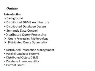
Outline • Introduction • Fragmentation(片段划分) • Horizontal fragmentation(水平划分) • Derived horizontal fragmentation(导出式水平划分) • Vertical fragmentation(垂直划分) • Allocation(片段分配)
Outline • Introduction • Fragmentation(片段划分) • Horizontal fragmentation(水平划分) • Derived horizontal fragmentation(导出式水平划分) • Vertical fragmentation(垂直划分) • Allocation(片段分配)
Distributed Database Design • The design of a distributed computer system involves making decisions on the placement of data and programs across the sites of a computer network. • In distributed DBMSs, such placement involves two things: • Placement of the DDBMS software • Placement of the applications that run on the database • The course concentrates on distribution of data. • The distribution of DDBMS and applications are given a priori.
Framework of Distribution Behavior of access pattern Dynamic Static Complete Information No sharing Data sharing Level of knowledge on access pattern behavior Data+ program sharing Partial Information Level of sharing
Design Strategies • Top-Down • Mostly in designing systems from scratch • Mostly in designing homogeneous systems • Bottom-up • When the databases already exist at a number of sites • Combining both
Top-Down Design Process User Input Requirement Analysis User Input Objectives View Integration View Design Conceptual Design Access Information ES’s GCS Distribution Design User Input LCS’s Physical Design LIS’s
Distribution Design Issues • Fragmentation • Why fragmentation at all? • How should we fragment? • How much should we fragment? • How to test correctness of decomposition? • Allocation • Necessary information required for fragmentation and allocation
Why Fragment? • Can’t we just distribute relations? • What is a reasonable unit of distribution? • Relation • Views are subsets of relations locality • Extra communication cost • Fragments of relations (sub-relations)
Fragmentation • Unit of distribution = unit of data application accesses • Reduce irrelevant data access • Facilitate intra-query concurrency over different fragments • Can be used with other performance enhancing methods (e.g., indexing and clustering) • Applications have conflicting requirements, making disjoint fragmentation a very hard problem • Multiple fragment access requires join or union • Semantic data control (integrity enforcement) could be very costly
About fragmentation • How should we fragment? • Vertical Fragments sub grouping of attributes • Horizontal Fragments sub grouping of tuples • Mixed/Hybrid Fragments combination of above two • How much to fragment? • Too little too much of irrelevant data access • Too much too much processing cost • Need to find suitable level of fragmentation
Correctness Criteria • Completeness no loss of data • Decomposition of relation R into fragments R1, R2, …, Rn is complete if and only if each data item in R can also be found in some Ri. • Reconstruction • If relation R is decomposed into fragments R1, R2, …, Rn then there should exist some relational operator such that R = 1 inRi • Disjointness • If relation R is decomposed into fragments R1, R2, …, Rn and data item di is in Rj, then di should not be in any other fragment Rk (k!=j).
Allocation Alternatives • Full Replication • Each fragment resides at each site • Partial Replication • Each fragment resides at some of the sites • Not-replicated (Partitioned) • Each fragment resides at only one site Q & A: What are the advantages and disadvantages?
Rule of Thumb for Allocation If number-of-read-only-queries is more than number-of-update-queries, then replication is advantageous, otherwise replication may cause problems.
Information Requirements • Four categories • Database information • Application information • Communication network information • Computer system information
Outline • Introduction • Fragmentation(片段划分) • Horizontal fragmentation(水平划分) • Derived horizontal fragmentation(导出式水平划分) • Vertical fragmentation(垂直划分) • Allocation(片段分配)
Fragmentation • Horizontal fragmentation (HF) • Primary horizontal fragmentation (PHF) • based on predicates accessing the relation • Derived horizontal fragmentation (DHF) • based on predicates being defined on another logically related relation We shall first study algorithm for horizontal fragmentation, and then study issues related to derived horizontal fragmentation. • Vertical fragmentation (VF) • Hybrid fragmentation (HVF)
PAY Title, Sal EMP PROJ Jno, Jname, Budget. Loc Eno,Ename, Title ASG Eno, Jno, Resp, Dur PHF Information Requirements • Database Information > links > Cardinality of each relation: card (R) L1 L2 L3
PHF Information Requirements (cont.) • Application Information 1 • Simple predicate:Given R(A1 , A2 , ..., An ), with each Ai having domain of values dom(Ai), a simple predicate pjis pj : AiValue where{<, >, , , } and Valuedom(Ai). Example Jname=“maintenance” Budget 200000 Follow ``80/20'' rule
PHF Information Requirements (cont.) • Application Information 2 • minterm predicate:Given R and a set of simple predicatesPr = {p1, p2, ..., pm}on R, the set of minterm predicates M= {m 1, m 2 , ..., m z } is defined as M = {mi| mi= PjPr p*j }, 1 iz, 1 j z where p*j = pjor ¬pj Example m1: (Jname=“maintenance”)(Budget 200000) m2: ¬(Jname=“maintenance”) (Budget 200000) m3: (Jname=“maintenance”) ¬(Budget 200000) m4: ¬(Jname=“maintenance”) ¬(Budget 200000)
PHF Information Requirements (cont.) • Application Information 3 • Minterm selectivity: sel (mi) • number of tuples of the relation that would be accessed by a user query specified according to a given minterm predicate. • Access frequency: acc (qi) • frequency with which user applications access data. If Q = {q1 , q2 , ..., qn } is the set of queries, acc (qi ) indicates access frequency of query qi in a given period.
Primary Horizontal Fragmentation • Each horizontal fragment Ri of relation R is defined by Ri = Fi (R), 1 iw, where Fiis a selection formula, which is (preferably) a minterm predicate. • A horizontal fragment Ri of relation R consists of all the tuples of R which satisfy a minterm predicate mi. • Given a set of minterm predicates M, there are as many as horizontal fragments of relation Ras there are minterm predicates. • Set of horizontal fragments also referred to as minterm fragments
PHF - Algorithm Input:A relation R, a set of simple predicates Pr Output: The set of fragments of R = {R1 , R2 , ..., Rw}, which obey the fragmentation rules. Preliminaries: • Pr should be complete • Pr should be minimal
Completeness of Simple Predicates • A set of simple predicatesPris said to be complete if and only if the accesses to the tuples of the minterm fragments defined on Pr requires that two tuples of the same minterm fragment have the same probability of being accessed by any application.
Completeness of Simple Predicates • Example: Applications: Q1: Find the projects at each location Q2: Find projects with budget less than $200,000 Predicates: Pr={ LOC=“Montreal”, LOC=“New York”, LOC=“Paris”} Pr={ LOC=“Montreal”, LOC=“New York”, LOC=“Paris”, BUDGET 2000000, BUDGET >200000} incomplete
Minimality of Simple Predicates • If a predicate influences how fragmentation is performed, (i.e., causes a fragment f to be further fragmented into, say, fi and fj), then there should be at least one application that accesses fi and fj differently. • In other words, the simple predicate should be relevant in determining a fragmentation. • If all the predicates of a set Prare relevant, then Pr is minimal.
Minimality of Simple Predicates Example Applications: Q1: Find the projects at each location Q2: Find projects with budget less than $200,000 Pr={ LOC=“Montreal”, LOC=“New York”, LOC=“Paris”, BUDGET 2000000, BUDGET >200000} minimal Pr={ LOC=“Montreal”, LOC=“New York”, LOC=“Paris”, BUDGET 2000000, BUDGET >200000, PNAME=“Instrumentation”} Minimal??
COM_MIN Algorithm Input:A relation R and a set of simple predicates Pr Output: A complete and minimal set of simple predicates Pr’ for Pr Rule 1: A relation or fragment is partitioned into at least two parts which are accessed differently by at least one application.
COM_MIN Algorithm (cont.) 1. Initialization • Find a pi Prsuch that pi partitions R according to Rule 1 • Set Pr’ = pi ; PrPr - pi ; F fi 2. Iteratively add predicates to Pr’ until it is complete • Find a pj Prsuch that pj partitions some fk defined according to minterm predicate over Pr’ according to Rule 1 • Pr’ pj ; Pr= Pr - pj ; F fj • If pk Pr’which is nonrelevant, then Pr ’ = Pr ’ - pk ; F F - fk
PHORIZONTAL Algorithm Make use of COM_MIN to perform fragmentation Input:A relation R and a set of simple predicates Pr Output: A set of minterm predicates M according to which relation Ris to be fragmented Steps: • Pr’ COM_MIN(R, Pr) • Determine the set M of minterm predicates • Determine the set I of implications among pi Pr’Eliminate the contradictory minterms from M
Contradictory Minterms • Given a minimal and complete set of simple predicates, containing n simple predicates • Not all the minterm fragments derived are valid • A fragment can be self contradictory because of implications among simple predicates. Example: Dom(Sal): [10000, 200000]; Dom(Loc) = {HK,SF} p1 : sal < 50000; p2 : Loc = HK; p3 : Loc = SF Note: p2(¬ p3 ); p3(¬ p2 ) the minterm p1p2p3 is self contradictory.
PHORIZONTAL Algorithm (cont.) Input: relationR and a set of simple predicates Pr Output: a set of minterm fragments M begin Pr’ = COM-MIN(R, Pr ); M = set of minterm predicates from Pr’ I = set of implications among piPr’ for eachmiM if mi is contradictory according to I then M = M mi end
PHF Example: PAY PAY Application: Check the salary info and determine raise Employee records kept at two sites ==> application runs at two sites Simple predicates: P1: SAL 30000, P2:SAL > 30000 Pr = {P1, P2}, which is complete and minimal Pr’ = Pr Minterm predicates: m1: (SAL 30000); m2: (SAL > 30000) PAY1 PAY2
PROJ PHF Example: PROJ Applications • Find the name and budget of projects given their locations • Issued at three sites • Access project information according to budget • One site access 200000; other accesses >200000 p1: LOC = “Montreal” p2 : LOC = “New York” p3 : LOC = “Paris” m1: LOC = “Montreal” BUDGET 200000 m2 : LOC = “Montreal” BUDGET > 200000 m3 : LOC = “New York” BUDGET 200000 m4 : LOC = “New York” BUDGET > 200000 m5 : LOC = “Paris” BUDGET 200000 M6 : LOC = “Paris” BUDGET > 200000 p4: BUDGET 200000 p5 : BUDGET > 200000
PROJ PHF Example: PROJ - Result PROJ1 PROJ2 PROJ4 m1: LOC = “Montreal” BUDGET 200000 m2 : LOC = “Montreal” BUDGET > 200000 m3 : LOC = “New York” BUDGET 200000 m4 : LOC = “New York” BUDGET > 200000 m5 : LOC = “Paris” BUDGET 200000 M6 : LOC = “Paris” BUDGET > 200000 PROJ6
PHF - Correctness • Completeness • Since Pr is complete and minimal, the selection predicates are complete • Reconstruction • If relation Ris fragmented into FR = {R1, R2, …, Rr} R = Ri FRRi • Disjointness • Minterm predicates that form the basis of fragmentation should be mutually exclusive
PAY Title, Sal EMP PROJ Jno, Jname, Budget. Loc Eno, Ename, Title ASG Eno, Jno, Resp, Dur DHF: Derived Horizontal Fragmentation DHF: Defined on a member relation according to a selection operation on its owner Owner relation Each link is an equijoin L1 L2 L3 Member relation
PAY2= SAL> 30000 PAY PAY1= SAL 30000 PAY PAY Title, Sal EMP Eno, Ename, Title L1 EMP2 = EMP PAY2 DHF – Example EMP1 = EMP PAY1 EMP DHF
DHF: Derived Horizontal Fragmentation • Let S be horizontally fragmented and let there be a link L with owner(L) = S, and member(L) = R, the derived horizontal fragments of R are defined as Ri= RSi , 1 iw where Si is the horizontal fragment of S, is the semijoin operator, and w is the maximum number of fragments • Inputs to derived horizontal fragmentation: • partitions of owner relation • member relation • the semijoin condition • The algorithm is straight forward.
DHF: Correctness • Completeness • primary horizontal fragmentation based on completeness of selection predicates. For derived horizontal fragmentation based on referential integrity • Reconstruction • Same as primary horizontal fragmentation (via union) • Disjointedness • Simple join graphs between the owner and the member fragments.
DHF: Issues • Multiple owners for a member relation; how should we derived horizontally fragmentsof a member relation? • There could be a chain of derived horizontal fragmentation.
Vertical Fragmentation (VF) • Has been studied within the centralized context • Vertical partitioning of a relation R produces fragments R1, R2, ..., Rm, each of which contains a subset of R's attributes as well as the primary key of R • The object of vertical fragmentation is to reduce irrelevant attribute access, and thus irrelevant data access • “Optimal” vertical fragmentation is one that minimizes the irrelevant data access for user applications
VF Two Approaches • Grouping: each individual attribute one fragment, at each step join some of the fragments until some criteria being satisfied • Attributes to fragments • Splitting: start with global relation, and generate beneficial partitions based on access behavior of the applications • Relations to fragments
Vertical Fragmentation • Overlapping fragments • grouping • Non-overlapping fragments • Splitting • We do not consider the replicated key attributes to be overlapping • Advantage • easier to enforce functional dependencies (for integrity checking)
VF Information Requirements • Application Information • Attribute affinities • A measure that indicates how closely related the attributes are • This is obtained from more primitive usage data • Attribute usage values • Given a set of queries Q = {q1 , q2, ..., qm}that will run on relation R (A1, A2, ..., An) use (qi, Aj) = 1 if attribute Aj is referenced by query qi 0 otherwise use (qi, .) can be defined accordingly.
VF Definition of use(qi, Aj) • Consider the following 4 queries for relation PROJ q1: SELECT BUDGET FROM PROJ WHERE PNO = val; q2: SELECT PNAME,BUDGET FROM PROJ; q3: SELECT PNAME FROM PROJWHERE LOC = val; q4: SELECT SUM(BUDGET) FROM PROJ WHERELOC=val; LetA1= PNO, A2= PNAME, A3 = BUDGET, A4 = LOC A1 A2 A3 A4 q1 q2 q3 q4
VF - Affinity Measureaff(Ai, Aj) • The attribute affinity measure between two attributes Aiand Aj of a relation R (A1, A2, ..., An) with respect to the set of applications Q = {q1 , q2, ..., qm} is defined as: Aff (Ai, Aj) = { k | use (qk, Ai)=1use (qk, Aj)=1}l refl (qk) * accl (qk) where refl(qk) is thenumber of accesses to attributes for each execution of applicationqkat site l; accl(qk)is theaccess frequency of queryqk at site l.
VF - Affinity Measureaff(Ai, Aj) S1 S2 S3 Assume each query in the previous example accesses the attributes once during each execution. Also assume the access frequency of query k at different sites is: then Aff (A1, A3) = 15*1 + 20*1 + 10*1 = 45 and the attribute affinity matrix AA is: q1 q2 q3 q4 A1 A2 A3 A4 A1 A2 A3 A4 A1 A2 A3 A4 q1 q2 q3 q4
AA Matrix for Vertical Fragmentation • This affinity matrix will be used to guide the fragmentation effort. The process involves first clustering together the attributes with high affinity for each other, and then splitting the relation accordingly.